Wold decomposition
A decomposition introduced by H. Wold in 1938 (see [a7]); see also [a5], [a8]. Standard references include [a6], [a3].
The Wold decomposition of a (weakly) stationary stochastic process  ,
,  , provides interesting insights in the structure of such processes and, in particular, is an important tool for forecasting (from an infinite past).
The main result can be summarized as:
1) Every (weakly) stationary process  can uniquely be decomposed as
 |
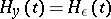
where the stationary processes  and
and  are obtained by causal linear transformations of
  (where "causal" means that, e.g.
  , only depends on
  ,
,  ),
),  and
and  are mutually uncorrelated,
  is linearly regular (i.e. the best linear least squares predictors converge to zero, if the forecasting horizon tends to infinity) and
  is linearly singular (i.e. the prediction errors for the best linear least squares predictors are zero).
2) Every linearly regular process  can be represented as
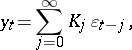 | (a1) |
 |
where  is white noise (i.e.
  ,
, 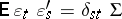 ) and
) and  is obtained by a causal linear transformation of
  .
.
The construction behind the Wold decomposition in the Hilbert space  spanned by the one-dimensional process variables
  is as follows: If
  denotes the subspace spanned by
  , then
  is obtained from projecting
  on the space
  , and
, and  is obtained as the perpendicular by projecting
  on the space
  spanned by
  . Thus
  is the innovation and the one-step-ahead prediction error for
  as well as for
  .
.
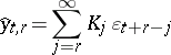
The implications of the above-mentioned results for (linear least squares) prediction are straightforward: Since  and
and  are orthogonal and since
  is the direct sum of
  and
and  , the prediction problem can be solved for the linearly regular and the linearly singular part separately, and for a linearly regular process
  ,
,  implies that the best linear least squares
  -step ahead predictor for
  is given by
 |
and thus the prediction error is
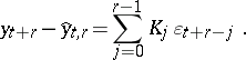 |
Thus, when the representation (a1) is available, the prediction problem for a linearly regular process can be solved.
The next problem is to obtain (a1) from the second moments of  (cf. also Moment). The problem of determining the coefficients
  of the Wold representation (a1) (or, equivalently, of determining the corresponding transfer function
 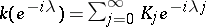 ) from the spectral density
 | (a2) |
(where the  denotes the conjugate transpose) of a linearly regular process
  , is called the spectral factorization problem. The following result holds:
3) A stationary process  with a spectral density
  , which is non-singular
  -a.e., is linearly regular if and only if
 |
In this case the factorization  in (a2) corresponding to the Wold representation (a1) satisfies the relation
 |
The most important special case is that of rational spectral densities; for such one has (see e.g. [a4]):
4) Any rational and  -a.e. non-singular spectral density
  can be uniquely factorized, such that
  (the extension of
  to
to  ) is rational, analytic within a circle containing the closed unit disc,
  ,
,  ,
,  (and thus corresponds to the Wold representation (a1)), and
  . Then (a1) is the solution of a stable and miniphase ARMA or a (linear) finite-dimensional state space system.
Evidently, the Wold representation (a1) relates stationary processes to linear systems with white noise inputs. Actually, Wold introduced (a1) as a joint representation for AR and MA systems (cf. also Mixed autoregressive moving-average process).
The Wold representation is used, e.g., for the construction of the state space of a linearly regular process and the construction of state space representations, see [a1], [a4]. As mentioned already, the case of rational transfer functions corresponding to stable and miniphase ARMA or (finite-dimensional) state space systems is by far the most important one. In this case there is a wide class of identification procedures available, which also give estimates of the coefficients  from finite data
  (see e.g. [a4]).
Another case is that of stationary long memory processes (see e.g. [a2]). In this case, in (a1),  , so that
  is infinity at frequency zero, which causes the long memory effect. Models of this kind, in particular so-called ARFIMA models, have attracted considerable attention in modern econometrics.
References
| [a1] | H. Akaike, "Stochastic theory of minimal realizations" IEEE Trans. Autom. Control , AC-19 (1974) pp. 667–674 |
| [a2] | C.W.J. Granger, R. Joyeux, "An introduction to long memory time series models and fractional differencing" J. Time Ser. Anal. , 1 (1980) pp. 15–39 |
| [a3] | E.J. Hannan, "Multiple time series" , Wiley (1970) |
| [a4] | E.J. Hannan, M. Deistler, "The statistical theory of linear systems" , Wiley (1988) |
| [a5] | A.N. Kolmogorov, "Stationary sequences in Hilbert space" Bull. Moscow State Univ. , 2 : 6 (1941) pp. 1–40 |
| [a6] | Y.A. Rozanov, "Stationary random processes" , Holden Day (1967) |
| [a7] | H. Wold, "Study in the analysis of stationary time series" , Almqvist and Wiksell (1954) (Edition: Second) |
| [a8] | V.N. Zasukhin, "On the theory of multidimensional stationary processes" Dokl. Akad. Nauk SSSR , 33 (1941) pp. 435–437 |
Wold decomposition. Encyclopedia of Mathematics. URL: http://encyclopediaofmath.org/index.php?title=Wold_decomposition&oldid=17678