|
|
| (235 intermediate revisions by the same user not shown) |
| Line 1: |
Line 1: |
| − | $\newcommand{\Om}{\Omega}
| + | <ref> [http://hea-www.harvard.edu/AstroStat http://hea-www.harvard.edu/AstroStat]; <nowiki> http://www.incagroup.org </nowiki>; <nowiki> http://astrostatistics.psu.edu </nowiki> </ref> |
| − | \newcommand{\F}{\mathcal F}
| |
| − | \newcommand{\B}{\mathcal B}
| |
| − | \newcommand{\M}{\mathcal M} $
| |
| − | A [[probability space]] is called '''standard''' if it satisfies the following equivalent conditions:
| |
| − | * it is [[Measure space#Isomorphism|almost isomorphic]] to the real line with some [[probability distribution]] (in other words, a [[Measure space#Completion|completed]] [[Borel measure|Borel]] [[probability measure]], that is, a [[Lebesgue–Stieltjes integral|Lebesgue–Stieltjes]] probability measure);
| |
| − | * it is a [[standard Borel space]] endowed with a [[probability measure]], completed, and possibly augmented with a [[Measure space#null|null set]];
| |
| − | * it is [[Measure space#Completion|complete]], [[Measure space#Perfect and standard|perfect]], and the [[Hilbert space#L2 space|corresponding Hilbert space]] is separable.
| |
| | | | |
| − | ====The isomorphism theorem==== | + | ====Notes==== |
| | + | <references /> |
| | | | |
| − | Every standard probability space consists of an [[Measure space#Atoms and continuity|atomic]] (discrete) part and an atomless (continuous) part (each part may be empty). The discrete part is finite or countable; here, all subsets are measurable, and the probability of each subset is the sum of probabilities of its elements.
| + | ------------------------------------------- |
| | | | |
| − | '''Theorem 1.''' All atomless standard probability spaces are mutually almost isomorphic.
| |
| | | | |
| − | That is, up to almost isomorphism we have "the" atomless standard probability space. Its "incarnations" include the spaces $\R^n$ with atomless probability distributions (be they [[Continuous distribution|absolutely continuous]] or [[Singular distribution|singular]]), as well as the set of all continuous functions $[0,\infty)\to\R$ with the [[Wiener measure]]. That is instructive: topological notions such as dimension, connectedness, compactness etc. do not apply to probability spaces.
| + | {| |
| − | | + | | A || B || C |
| − | ====Measure preserving injections====
| + | |- |
| | + | | X || Y || Z |
| | + | |} |
| | | | |
| − | Here is another important fact in two equivalent forms.
| |
| | | | |
| − | '''Theorem 2a.''' If a bijective map between standard probability spaces is measure preserving then the inverse map is also measure preserving.
| |
| | | | |
| − | '''Theorem 2b.''' If $(\Om,\F,P)$ is a standard probability space and $\F_1\subset\F$ a sub-σ-field such that $(\Om,\F_1,P|_{\F_1})$ is standard then $\F_1=\F$.
| + | ----------------------------------------- |
| | + | ----------------------------------------- |
| | | | |
| − | Recall a topological fact similar to Theorem 2: if a bijective map between compact Hausdorff topological spaces is continuous then the inverse map is also continuous. Moreover, if a Hausdorff topology is weaker than a compact topology then these two topologies are equal, which has the following Borel-space counterpart stronger than Theorem 2 (in three equivalent forms).
| + | $\newcommand*{\longhookrightarrow}{\lhook\joinrel\relbar\joinrel\rightarrow}$ |
| | | | |
| − | '''Theorem 3a.''' If a bijective map from a standard probability space to a countably separated probability space is measure preserving then the inverse map is also measure preserving.
| + | <asy> |
| | + | size(100,100); |
| | + | label(scale(1.7)*'$T(\\Sigma)\hookrightarrow T(\\Sigma,X)$',(0,0)); |
| | + | </asy> |
| | | | |
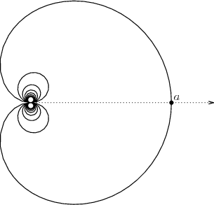
| − | (In general, the inverse to a bijective measure preserving map is measure preserving provided that it is measurable.) | + | <asy> |
| | + | size(220,220); |
| | | | |
| − | '''Theorem 3b.''' If $(\Om,\F,P)$ is a standard probability space and $\F_1\subset\F$ is a countably separated sub-σ-field then $(\Om,\F,P)$ is the completion of $(\Om,\F_1,P|_{\F_1})$.
| + | import math; |
| | | | |
| − | -------------------------------------------------------
| + | int kmax=40; |
| | | | |
| | + | guide g; |
| | + | for (int k=-kmax; k<=kmax; ++k) { |
| | + | real phi = 0.2*k*pi; |
| | + | real rho = 1; |
| | + | if (k!=0) { |
| | + | rho = sin(phi)/phi; |
| | + | } |
| | + | pair z=rho*expi(phi); |
| | + | g=g..z; |
| | + | } |
| | + | |
| | + | draw (g); |
| | | | |
| − | ''Non-example.'' The set $[0,1]^\R$ of all functions $\R\to[0,1]$ with the product of Lebesgue measures is a nonstandard probability space.
| + | defaultpen(0.75); |
| | + | draw ( (0,0)--(1.3,0), dotted, Arrow(SimpleHead,5) ); |
| | + | dot ( (1,0) ); |
| | + | label ( "$a$", (1,0), NE ); |
| | | | |
| − | '''Definition 1a.''' A probability space $(\Om,\F,P)$ is ''standard'' if it is [[Measure space#complete|complete]] and there exist a subset $\Om_1\subset\Om$ and a σ-field (in other words, σ-algebra) $\B$ on $\Om_1$ such that $(\Om_1,\B)$ is a standard Borel space and every set of $\F$ is [[Measure space#almost|almost equal]] to a set of $\B$. (See {{Cite|I|Sect. 2.4}}.) (Clearly, $\Om_1$ must be of [[Measure space#full|full measure]].)
| + | </asy> |
| − | | |
| − | '''Definition 1b''' (equivalent). A probability space $(\Om,\F,P)$ is ''standard'' if it is complete, [[Measure space#perfect|perfect]] and countably separated mod 0 in the following sense: some subset of full measure, treated as a [[Measurable space#subspace|subspace]] of the measurable space $(\Om,\F)$, is a [[Measurable space#separated|countably separated]] measurable space.
| |
| − | | |
| − | (See {{Cite|I|Sect. 3.1}} for a proof of equivalence of these definitions.)
| |
| − | | |
| − | ====On terminology====
| |
| − | | |
| − | Also "Lebesgue-Rokhlin space" and "[[Lebesgue space]]".
| |
| − | | |
| − | In {{Cite|M|Sect. 6}} universally measurable spaces are called metrically standard Borel spaces.
| |
| − | | |
| − | In {{Cite|K|Sect. 21.D}} universally measurable subsets of a standard (rather than arbitrary) measurable space are defined.
| |
| − | | |
| − | In {{Cite|N|Sect. 1.1}} an absolute measurable space is defined as a separable metrizable topological space such that every its homeomorphic image in every such space (with the Borel σ-algebra) is a universally measurable subset. The corresponding measurable space (with the Borel σ-algebra) is also called an absolute measurable space in {{Cite|N|Sect. B.2}}.
| |
| − | | |
| − | ====References====
| |
| − | | |
| − | {|
| |
| − | |valign="top"|{{Ref|I}}|| Kiyosi Itô, "Introduction to probability theory", Cambridge (1984). {{MR|0777504}} {{ZBL|0545.60001}}
| |
| − | |-
| |
| − | |valign="top"|{{Ref|B}}|| V.I. Bogachev, "Measure theory", Springer-Verlag (2007). {{MR|2267655}} {{ZBL|1120.28001}}
| |
| − | |-
| |
| − | |valign="top"|{{Ref|C}}|| Donald L. Cohn, "Measure theory", Birkhäuser (1993). {{MR|1454121}} {{ZBL|0860.28001}}
| |
| − | |-
| |
| − | |valign="top"|{{Ref|D}}|| Richard M. Dudley, "Real analysis and probability", Wadsworth&Brooks/Cole (1989). {{MR|0982264}} {{ZBL|0686.60001}}
| |
| − | |-
| |
| − | |valign="top"|{{Ref|M}}|| George W. Mackey, "Borel structure in groups and their duals", ''Trans. Amer. Math. Soc.'' '''85''' (1957), 134–165. {{MR|0089999}} {{ZBL|0082.11201}}
| |
| − | |-
| |
| − | |valign="top"|{{Ref|K}}|| Alexander S. Kechris, "Classical descriptive set theory", Springer-Verlag (1995). {{MR|1321597}} {{ZBL|0819.04002}}
| |
| − | |-
| |
| − | |valign="top"|{{Ref|N}}|| Togo Nishiura, "Absolute measurable spaces", Cambridge (2008). {{MR|2426721}} {{ZBL|1151.54001}}
| |
| − | |}
| |