Difference between revisions of "Trigonometric sums, method of"
Ulf Rehmann (talk | contribs) m (tex encoded by computer) |
Ulf Rehmann (talk | contribs) m (Undo revision 49039 by Ulf Rehmann (talk)) Tag: Undo |
||
| Line 1: | Line 1: | ||
| − | |||
| − | |||
| − | |||
| − | |||
| − | |||
| − | |||
| − | |||
| − | |||
| − | |||
| − | |||
| − | |||
| − | |||
One of the general methods in [[Analytic number theory|analytic number theory]]. Two problems in number theory required for their solution the creation of the method of trigonometric sums: the problem of the distribution of the fractional parts of a polynomial (cf. [[Fractional part of a number|Fractional part of a number]]), and the problem of representing a positive integer as the sum of terms of a specified type (additive problems of number theory, cf. [[Additive number theory|Additive number theory]]). | One of the general methods in [[Analytic number theory|analytic number theory]]. Two problems in number theory required for their solution the creation of the method of trigonometric sums: the problem of the distribution of the fractional parts of a polynomial (cf. [[Fractional part of a number|Fractional part of a number]]), and the problem of representing a positive integer as the sum of terms of a specified type (additive problems of number theory, cf. [[Additive number theory|Additive number theory]]). | ||
| − | Let | + | Let <img align="absmiddle" border="0" src="https://www.encyclopediaofmath.org/legacyimages/t/t094/t094260/t0942601.png" /> be a real-valued function, <img align="absmiddle" border="0" src="https://www.encyclopediaofmath.org/legacyimages/t/t094/t094260/t0942602.png" />, <img align="absmiddle" border="0" src="https://www.encyclopediaofmath.org/legacyimages/t/t094/t094260/t0942603.png" />. One says that the fractional parts of <img align="absmiddle" border="0" src="https://www.encyclopediaofmath.org/legacyimages/t/t094/t094260/t0942604.png" /> are uniformly distributed if for any <img align="absmiddle" border="0" src="https://www.encyclopediaofmath.org/legacyimages/t/t094/t094260/t0942605.png" /> and <img align="absmiddle" border="0" src="https://www.encyclopediaofmath.org/legacyimages/t/t094/t094260/t0942606.png" />, <img align="absmiddle" border="0" src="https://www.encyclopediaofmath.org/legacyimages/t/t094/t094260/t0942607.png" />, the number <img align="absmiddle" border="0" src="https://www.encyclopediaofmath.org/legacyimages/t/t094/t094260/t0942608.png" /> of fractional parts of <img align="absmiddle" border="0" src="https://www.encyclopediaofmath.org/legacyimages/t/t094/t094260/t0942609.png" /> occurring in the interval <img align="absmiddle" border="0" src="https://www.encyclopediaofmath.org/legacyimages/t/t094/t094260/t09426010.png" /> is proportional to the length of this interval, that is, |
| − | be a real-valued function, | ||
| − | |||
| − | One says that the fractional parts of | ||
| − | are uniformly distributed if for any | ||
| − | and | ||
| − | |||
| − | the number | ||
| − | of fractional parts of | ||
| − | occurring in the interval | ||
| − | is proportional to the length of this interval, that is, | ||
| − | + | <table class="eq" style="width:100%;"> <tr><td valign="top" style="width:94%;text-align:center;"><img align="absmiddle" border="0" src="https://www.encyclopediaofmath.org/legacyimages/t/t094/t094260/t09426011.png" /></td> </tr></table> | |
| − | |||
| − | |||
| − | Now, let | + | Now, let <img align="absmiddle" border="0" src="https://www.encyclopediaofmath.org/legacyimages/t/t094/t094260/t09426012.png" /> be the characteristic function of the interval <img align="absmiddle" border="0" src="https://www.encyclopediaofmath.org/legacyimages/t/t094/t094260/t09426013.png" />, that is, |
| − | be the characteristic function of the interval | ||
| − | that is, | ||
| − | + | <table class="eq" style="width:100%;"> <tr><td valign="top" style="width:94%;text-align:center;"><img align="absmiddle" border="0" src="https://www.encyclopediaofmath.org/legacyimages/t/t094/t094260/t09426014.png" /></td> </tr></table> | |
| − | |||
| − | Extending | + | Extending <img align="absmiddle" border="0" src="https://www.encyclopediaofmath.org/legacyimages/t/t094/t094260/t09426015.png" /> periodically to the entire real axis, that is, setting <img align="absmiddle" border="0" src="https://www.encyclopediaofmath.org/legacyimages/t/t094/t094260/t09426016.png" />, one obtains |
| − | periodically to the entire real axis, that is, setting | ||
| − | one obtains | ||
| − | + | <table class="eq" style="width:100%;"> <tr><td valign="top" style="width:94%;text-align:center;"><img align="absmiddle" border="0" src="https://www.encyclopediaofmath.org/legacyimages/t/t094/t094260/t09426017.png" /></td> </tr></table> | |
| − | |||
| − | |||
| − | Expanding | + | Expanding <img align="absmiddle" border="0" src="https://www.encyclopediaofmath.org/legacyimages/t/t094/t094260/t09426018.png" /> in a [[Fourier series|Fourier series]], one obtains |
| − | in a [[Fourier series|Fourier series]], one obtains | ||
| − | + | <table class="eq" style="width:100%;"> <tr><td valign="top" style="width:94%;text-align:center;"><img align="absmiddle" border="0" src="https://www.encyclopediaofmath.org/legacyimages/t/t094/t094260/t09426019.png" /></td> </tr></table> | |
| − | |||
| − | |||
| − | |||
| − | |||
Thus, | Thus, | ||
| − | + | <table class="eq" style="width:100%;"> <tr><td valign="top" style="width:94%;text-align:center;"><img align="absmiddle" border="0" src="https://www.encyclopediaofmath.org/legacyimages/t/t094/t094260/t09426020.png" /></td> <td valign="top" style="width:5%;text-align:right;">(1)</td></tr></table> | |
| − | |||
| − | |||
| − | |||
| − | |||
| − | |||
| − | |||
| − | |||
| − | |||
| − | This last relation is not true in general, since there may be | + | This last relation is not true in general, since there may be <img align="absmiddle" border="0" src="https://www.encyclopediaofmath.org/legacyimages/t/t094/t094260/t09426021.png" /> such that <img align="absmiddle" border="0" src="https://www.encyclopediaofmath.org/legacyimages/t/t094/t094260/t09426022.png" /> or <img align="absmiddle" border="0" src="https://www.encyclopediaofmath.org/legacyimages/t/t094/t094260/t09426023.png" />; but <img align="absmiddle" border="0" src="https://www.encyclopediaofmath.org/legacyimages/t/t094/t094260/t09426024.png" /> and <img align="absmiddle" border="0" src="https://www.encyclopediaofmath.org/legacyimages/t/t094/t094260/t09426025.png" /> can be replaced by <img align="absmiddle" border="0" src="https://www.encyclopediaofmath.org/legacyimages/t/t094/t094260/t09426026.png" /> and <img align="absmiddle" border="0" src="https://www.encyclopediaofmath.org/legacyimages/t/t094/t094260/t09426027.png" /> that are close and are such that for all <img align="absmiddle" border="0" src="https://www.encyclopediaofmath.org/legacyimages/t/t094/t094260/t09426028.png" />, <img align="absmiddle" border="0" src="https://www.encyclopediaofmath.org/legacyimages/t/t094/t094260/t09426029.png" /> and <img align="absmiddle" border="0" src="https://www.encyclopediaofmath.org/legacyimages/t/t094/t094260/t09426030.png" />; the precision of the formula is practically unchanged by this substitution, and the formula becomes true. In exactly the same way, the function <img align="absmiddle" border="0" src="https://www.encyclopediaofmath.org/legacyimages/t/t094/t094260/t09426031.png" /> can be "smoothed out" ( "corrected" ), so that the magnitude of <img align="absmiddle" border="0" src="https://www.encyclopediaofmath.org/legacyimages/t/t094/t094260/t09426032.png" /> is practically unchanged and the coefficients <img align="absmiddle" border="0" src="https://www.encyclopediaofmath.org/legacyimages/t/t094/t094260/t09426033.png" /> of the Fourier series rapidly decrease as <img align="absmiddle" border="0" src="https://www.encyclopediaofmath.org/legacyimages/t/t094/t094260/t09426034.png" /> increases, that is, so that the series |
| − | such that | ||
| − | or | ||
| − | but | ||
| − | and | ||
| − | can be replaced by | ||
| − | and | ||
| − | that are close and are such that for all | ||
| − | |||
| − | and | ||
| − | the precision of the formula is practically unchanged by this substitution, and the formula becomes true. In exactly the same way, the function | ||
| − | can be "smoothed out" ( "corrected" ), so that the magnitude of | ||
| − | is practically unchanged and the coefficients | ||
| − | of the Fourier series rapidly decrease as | ||
| − | increases, that is, so that the series | ||
| − | + | <table class="eq" style="width:100%;"> <tr><td valign="top" style="width:94%;text-align:center;"><img align="absmiddle" border="0" src="https://www.encyclopediaofmath.org/legacyimages/t/t094/t094260/t09426035.png" /></td> </tr></table> | |
| − | |||
| − | |||
rapidly converges. | rapidly converges. | ||
| − | The second term in equation (1) does not exceed | + | The second term in equation (1) does not exceed <img align="absmiddle" border="0" src="https://www.encyclopediaofmath.org/legacyimages/t/t094/t094260/t09426036.png" /> in absolute value, where |
| − | in absolute value, where | ||
| − | + | <table class="eq" style="width:100%;"> <tr><td valign="top" style="width:94%;text-align:center;"><img align="absmiddle" border="0" src="https://www.encyclopediaofmath.org/legacyimages/t/t094/t094260/t09426037.png" /></td> </tr></table> | |
| − | |||
| − | |||
| − | |||
| − | |||
| − | |||
| − | |||
| − | |||
If it is known that | If it is known that | ||
| − | + | <table class="eq" style="width:100%;"> <tr><td valign="top" style="width:94%;text-align:center;"><img align="absmiddle" border="0" src="https://www.encyclopediaofmath.org/legacyimages/t/t094/t094260/t09426038.png" /></td> <td valign="top" style="width:5%;text-align:right;">(2)</td></tr></table> | |
| − | |||
| − | |||
| − | |||
| − | where | + | where <img align="absmiddle" border="0" src="https://www.encyclopediaofmath.org/legacyimages/t/t094/t094260/t09426039.png" /> as <img align="absmiddle" border="0" src="https://www.encyclopediaofmath.org/legacyimages/t/t094/t094260/t09426040.png" />, then one obtains for <img align="absmiddle" border="0" src="https://www.encyclopediaofmath.org/legacyimages/t/t094/t094260/t09426041.png" />: |
| − | as | ||
| − | then one obtains for | ||
| − | + | <table class="eq" style="width:100%;"> <tr><td valign="top" style="width:94%;text-align:center;"><img align="absmiddle" border="0" src="https://www.encyclopediaofmath.org/legacyimages/t/t094/t094260/t09426042.png" /></td> </tr></table> | |
| − | |||
| − | |||
| − | |||
| − | that is, the fractional parts of | + | that is, the fractional parts of <img align="absmiddle" border="0" src="https://www.encyclopediaofmath.org/legacyimages/t/t094/t094260/t09426043.png" /> are uniformly distributed. Thus, one must provide an upper bound of the modulus of a trigonometric sum. Since each term in <img align="absmiddle" border="0" src="https://www.encyclopediaofmath.org/legacyimages/t/t094/t094260/t09426044.png" /> is equal to 1 in modulus, a trivial bound of <img align="absmiddle" border="0" src="https://www.encyclopediaofmath.org/legacyimages/t/t094/t094260/t09426045.png" /> is <img align="absmiddle" border="0" src="https://www.encyclopediaofmath.org/legacyimages/t/t094/t094260/t09426046.png" />, that is, the number of terms of the sum <img align="absmiddle" border="0" src="https://www.encyclopediaofmath.org/legacyimages/t/t094/t094260/t09426047.png" />. An estimate of the form (2) is said to be non-trivial if <img align="absmiddle" border="0" src="https://www.encyclopediaofmath.org/legacyimages/t/t094/t094260/t09426048.png" />, and <img align="absmiddle" border="0" src="https://www.encyclopediaofmath.org/legacyimages/t/t094/t094260/t09426049.png" /> is called a reducing factor. |
| − | are uniformly distributed. Thus, one must provide an upper bound of the modulus of a trigonometric sum. Since each term in | ||
| − | is equal to 1 in modulus, a trivial bound of | ||
| − | is | ||
| − | that is, the number of terms of the sum | ||
| − | An estimate of the form (2) is said to be non-trivial if | ||
| − | and | ||
| − | is called a reducing factor. | ||
| − | In the problem of the fractional parts of | + | In the problem of the fractional parts of <img align="absmiddle" border="0" src="https://www.encyclopediaofmath.org/legacyimages/t/t094/t094260/t09426050.png" />, one can, by smoothing <img align="absmiddle" border="0" src="https://www.encyclopediaofmath.org/legacyimages/t/t094/t094260/t09426051.png" /> if necessary, merely require that the estimate (2) be obtained for "a relatively small" number of values of <img align="absmiddle" border="0" src="https://www.encyclopediaofmath.org/legacyimages/t/t094/t094260/t09426052.png" />, for example, for <img align="absmiddle" border="0" src="https://www.encyclopediaofmath.org/legacyimages/t/t094/t094260/t09426053.png" /> in the interval <img align="absmiddle" border="0" src="https://www.encyclopediaofmath.org/legacyimages/t/t094/t094260/t09426054.png" />, where <img align="absmiddle" border="0" src="https://www.encyclopediaofmath.org/legacyimages/t/t094/t094260/t09426055.png" /> is some constant. |
| − | one can, by smoothing | ||
| − | if necessary, merely require that the estimate (2) be obtained for "a relatively small" number of values of | ||
| − | for example, for | ||
| − | in the interval | ||
| − | where | ||
| − | is some constant. | ||
A similar approach is applied in the derivation of an asymptotic formula for the sum | A similar approach is applied in the derivation of an asymptotic formula for the sum | ||
| − | + | <table class="eq" style="width:100%;"> <tr><td valign="top" style="width:94%;text-align:center;"><img align="absmiddle" border="0" src="https://www.encyclopediaofmath.org/legacyimages/t/t094/t094260/t09426056.png" /></td> </tr></table> | |
| − | |||
| − | |||
| − | |||
which occurs in problems on the number of integer points in regions of the plane and in space. | which occurs in problems on the number of integer points in regions of the plane and in space. | ||
| Line 143: | Line 51: | ||
In additive problems of number theory, trigonometric sums occur in the following way. | In additive problems of number theory, trigonometric sums occur in the following way. | ||
| − | The following formula holds for an integer | + | The following formula holds for an integer <img align="absmiddle" border="0" src="https://www.encyclopediaofmath.org/legacyimages/t/t094/t094260/t09426057.png" />: |
| − | + | <table class="eq" style="width:100%;"> <tr><td valign="top" style="width:94%;text-align:center;"><img align="absmiddle" border="0" src="https://www.encyclopediaofmath.org/legacyimages/t/t094/t094260/t09426058.png" /></td> </tr></table> | |
| − | |||
| − | Therefore, if | + | Therefore, if <img align="absmiddle" border="0" src="https://www.encyclopediaofmath.org/legacyimages/t/t094/t094260/t09426059.png" /> denotes the number of solutions of the equation |
| − | denotes the number of solutions of the equation | ||
| − | + | <table class="eq" style="width:100%;"> <tr><td valign="top" style="width:94%;text-align:center;"><img align="absmiddle" border="0" src="https://www.encyclopediaofmath.org/legacyimages/t/t094/t094260/t09426060.png" /></td> </tr></table> | |
| − | |||
| − | |||
| − | |||
| − | |||
| − | where the | + | where the <img align="absmiddle" border="0" src="https://www.encyclopediaofmath.org/legacyimages/t/t094/t094260/t09426061.png" /> are certain sets of natural numbers, then |
| − | are certain sets of natural numbers, then | ||
| − | + | <table class="eq" style="width:100%;"> <tr><td valign="top" style="width:94%;text-align:center;"><img align="absmiddle" border="0" src="https://www.encyclopediaofmath.org/legacyimages/t/t094/t094260/t09426062.png" /></td> </tr></table> | |
| − | |||
| − | |||
| − | |||
| − | |||
where | where | ||
| − | + | <table class="eq" style="width:100%;"> <tr><td valign="top" style="width:94%;text-align:center;"><img align="absmiddle" border="0" src="https://www.encyclopediaofmath.org/legacyimages/t/t094/t094260/t09426063.png" /></td> </tr></table> | |
| − | |||
| − | |||
| − | |||
| − | |||
| − | |||
| − | In particular, by setting | + | In particular, by setting <img align="absmiddle" border="0" src="https://www.encyclopediaofmath.org/legacyimages/t/t094/t094260/t09426064.png" /> one obtains the [[Waring problem|Waring problem]]; for <img align="absmiddle" border="0" src="https://www.encyclopediaofmath.org/legacyimages/t/t094/t094260/t09426065.png" />, <img align="absmiddle" border="0" src="https://www.encyclopediaofmath.org/legacyimages/t/t094/t094260/t09426066.png" />, the ternary [[Goldbach problem|Goldbach problem]], etc. As in the problem on the distribution of fractional parts, the main question here is that of finding an upper bound of the modulus of <img align="absmiddle" border="0" src="https://www.encyclopediaofmath.org/legacyimages/t/t094/t094260/t09426067.png" />, that is, the question of an upper bound of <img align="absmiddle" border="0" src="https://www.encyclopediaofmath.org/legacyimages/t/t094/t094260/t09426068.png" />. |
| − | one obtains the [[Waring problem|Waring problem]]; for | ||
| − | |||
| − | the ternary [[Goldbach problem|Goldbach problem]], etc. As in the problem on the distribution of fractional parts, the main question here is that of finding an upper bound of the modulus of | ||
| − | that is, the question of an upper bound of | ||
Thus, a variety of problems in number theory can be formulated uniformly in the language of trigonometric sums. | Thus, a variety of problems in number theory can be formulated uniformly in the language of trigonometric sums. | ||
| Line 185: | Line 73: | ||
The first non-trivial trigonometric sum appeared in the work of C.F. Gauss (1811) in one of his proofs of the reciprocity law for quadratic residues (cf. [[Quadratic reciprocity law|Quadratic reciprocity law]]): | The first non-trivial trigonometric sum appeared in the work of C.F. Gauss (1811) in one of his proofs of the reciprocity law for quadratic residues (cf. [[Quadratic reciprocity law|Quadratic reciprocity law]]): | ||
| − | + | <table class="eq" style="width:100%;"> <tr><td valign="top" style="width:94%;text-align:center;"><img align="absmiddle" border="0" src="https://www.encyclopediaofmath.org/legacyimages/t/t094/t094260/t09426069.png" /></td> </tr></table> | |
| − | |||
| − | |||
| − | |||
| − | |||
| − | |||
| − | Gauss calculated the precise value of | + | Gauss calculated the precise value of <img align="absmiddle" border="0" src="https://www.encyclopediaofmath.org/legacyimages/t/t094/t094260/t09426070.png" />: |
| − | + | <table class="eq" style="width:100%;"> <tr><td valign="top" style="width:94%;text-align:center;"><img align="absmiddle" border="0" src="https://www.encyclopediaofmath.org/legacyimages/t/t094/t094260/t09426071.png" /></td> </tr></table> | |
| − | |||
A whole series of independent articles applying trigonometric sums appeared at the beginning of the 20th century. | A whole series of independent articles applying trigonometric sums appeared at the beginning of the 20th century. | ||
| Line 201: | Line 83: | ||
H. Weyl studied the distribution of the fractional parts of a polynomial | H. Weyl studied the distribution of the fractional parts of a polynomial | ||
| − | + | <table class="eq" style="width:100%;"> <tr><td valign="top" style="width:94%;text-align:center;"><img align="absmiddle" border="0" src="https://www.encyclopediaofmath.org/legacyimages/t/t094/t094260/t09426072.png" /></td> </tr></table> | |
| − | |||
| − | |||
| − | with real coefficients | + | with real coefficients <img align="absmiddle" border="0" src="https://www.encyclopediaofmath.org/legacyimages/t/t094/t094260/t09426073.png" />, and considered sums <img align="absmiddle" border="0" src="https://www.encyclopediaofmath.org/legacyimages/t/t094/t094260/t09426074.png" /> with a function <img align="absmiddle" border="0" src="https://www.encyclopediaofmath.org/legacyimages/t/t094/t094260/t09426075.png" /> of the form <img align="absmiddle" border="0" src="https://www.encyclopediaofmath.org/legacyimages/t/t094/t094260/t09426076.png" />, where <img align="absmiddle" border="0" src="https://www.encyclopediaofmath.org/legacyimages/t/t094/t094260/t09426077.png" /> is a non-zero integer. I.M. Vinogradov (1917), in the study of the distribution of integer points in regions of the plane and in space, considered sums <img align="absmiddle" border="0" src="https://www.encyclopediaofmath.org/legacyimages/t/t094/t094260/t09426078.png" /> with a function <img align="absmiddle" border="0" src="https://www.encyclopediaofmath.org/legacyimages/t/t094/t094260/t09426079.png" /> of which it was required only that its second derivative satisfy the conditions |
| − | and considered sums | ||
| − | with a function | ||
| − | of the form | ||
| − | where | ||
| − | is a non-zero integer. I.M. Vinogradov (1917), in the study of the distribution of integer points in regions of the plane and in space, considered sums | ||
| − | with a function | ||
| − | of which it was required only that its second derivative satisfy the conditions | ||
| − | + | <table class="eq" style="width:100%;"> <tr><td valign="top" style="width:94%;text-align:center;"><img align="absmiddle" border="0" src="https://www.encyclopediaofmath.org/legacyimages/t/t094/t094260/t09426080.png" /></td> </tr></table> | |
| − | |||
| − | |||
| − | |||
| − | |||
| − | |||
| − | |||
| − | |||
| − | |||
| − | where | + | where <img align="absmiddle" border="0" src="https://www.encyclopediaofmath.org/legacyimages/t/t094/t094260/t09426081.png" /> are absolute positive constants and <img align="absmiddle" border="0" src="https://www.encyclopediaofmath.org/legacyimages/t/t094/t094260/t09426082.png" />. G.H. Hardy and J.E. Littlewood (1918), having obtained an approximate functional equation of the Riemann zeta-function, considered the sum <img align="absmiddle" border="0" src="https://www.encyclopediaofmath.org/legacyimages/t/t094/t094260/t09426083.png" /> with a function <img align="absmiddle" border="0" src="https://www.encyclopediaofmath.org/legacyimages/t/t094/t094260/t09426084.png" /> of the form |
| − | are absolute positive constants and | ||
| − | G.H. Hardy and J.E. Littlewood (1918), having obtained an approximate functional equation of the Riemann zeta-function, considered the sum | ||
| − | with a function | ||
| − | of the form | ||
| − | + | <table class="eq" style="width:100%;"> <tr><td valign="top" style="width:94%;text-align:center;"><img align="absmiddle" border="0" src="https://www.encyclopediaofmath.org/legacyimages/t/t094/t094260/t09426085.png" /></td> </tr></table> | |
| − | |||
| − | |||
| − | where | + | where <img align="absmiddle" border="0" src="https://www.encyclopediaofmath.org/legacyimages/t/t094/t094260/t09426086.png" /> is a real parameter, <img align="absmiddle" border="0" src="https://www.encyclopediaofmath.org/legacyimages/t/t094/t094260/t09426087.png" />. |
| − | is a real parameter, | ||
| − | In all these papers it was required to find a best possible bound of the modulus of the sum | + | In all these papers it was required to find a best possible bound of the modulus of the sum <img align="absmiddle" border="0" src="https://www.encyclopediaofmath.org/legacyimages/t/t094/t094260/t09426088.png" />. |
The general scheme for studying these problems in number theory by the method of trigonometric sums is as follows. One writes down the exact formula expressing the number of solutions of the equation under study, or the number of fractional parts of the function under study occurring in a given interval, or the number of integer points in a given region, in the form of an integral of trigonometric sums or in the form of a series whose coefficients are trigonometric sums. The exact formula is expressed as the sum of two terms, the principal and the secondary term (e.g. if one is considering the Fourier series of the characteristic function of an interval, then the principal term is obtained from the zero coefficient of the Fourier series); the principal term supplies the principal term of the asymptotic formula, the secondary term supplies the remainder term. In additive problems such as the Waring problem, the Goldbach problem, etc., the principal term is studied by a method close to the circle method of Hardy–Littlewood–Ramanujan (this method is called the [[Circle method|circle method]] in the form of Vinogradov trigonometric sums). In the majority of other problems (the distribution of fractional parts, integer points in regions, etc.), the principal term is obtained trivially. There now arises the problem of estimating the remainder term, and if it can be proved that it is a quantity of smaller order than the principal term, then the asymptotic formula has been proved. | The general scheme for studying these problems in number theory by the method of trigonometric sums is as follows. One writes down the exact formula expressing the number of solutions of the equation under study, or the number of fractional parts of the function under study occurring in a given interval, or the number of integer points in a given region, in the form of an integral of trigonometric sums or in the form of a series whose coefficients are trigonometric sums. The exact formula is expressed as the sum of two terms, the principal and the secondary term (e.g. if one is considering the Fourier series of the characteristic function of an interval, then the principal term is obtained from the zero coefficient of the Fourier series); the principal term supplies the principal term of the asymptotic formula, the secondary term supplies the remainder term. In additive problems such as the Waring problem, the Goldbach problem, etc., the principal term is studied by a method close to the circle method of Hardy–Littlewood–Ramanujan (this method is called the [[Circle method|circle method]] in the form of Vinogradov trigonometric sums). In the majority of other problems (the distribution of fractional parts, integer points in regions, etc.), the principal term is obtained trivially. There now arises the problem of estimating the remainder term, and if it can be proved that it is a quantity of smaller order than the principal term, then the asymptotic formula has been proved. | ||
Revision as of 14:53, 7 June 2020
One of the general methods in analytic number theory. Two problems in number theory required for their solution the creation of the method of trigonometric sums: the problem of the distribution of the fractional parts of a polynomial (cf. Fractional part of a number), and the problem of representing a positive integer as the sum of terms of a specified type (additive problems of number theory, cf. Additive number theory).
Let  be a real-valued function,
  ,
,  . One says that the fractional parts of
  are uniformly distributed if for any
  and
and  ,
,  , the number
  of fractional parts of
  occurring in the interval
  is proportional to the length of this interval, that is,
 |
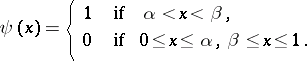
Now, let  be the characteristic function of the interval
  , that is,
 |
Extending  periodically to the entire real axis, that is, setting
  , one obtains
 |
Expanding  in a Fourier series, one obtains
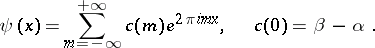 |
Thus,
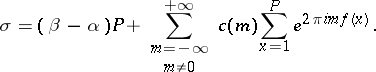 | (1) |
This last relation is not true in general, since there may be  such that
  or
or  ; but
; but  and
and  can be replaced by
  and
and  that are close and are such that for all
  ,
,  and
and  ; the precision of the formula is practically unchanged by this substitution, and the formula becomes true. In exactly the same way, the function
  can be "smoothed out" ( "corrected" ), so that the magnitude of
  is practically unchanged and the coefficients
  of the Fourier series rapidly decrease as
  increases, that is, so that the series
 |
rapidly converges.
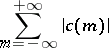
The second term in equation (1) does not exceed  in absolute value, where
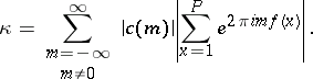 |
If it is known that
 | (2) |
where  as
as  , then one obtains for
  :
:
 |
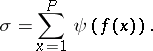
that is, the fractional parts of  are uniformly distributed. Thus, one must provide an upper bound of the modulus of a trigonometric sum. Since each term in
  is equal to 1 in modulus, a trivial bound of
  is
is  , that is, the number of terms of the sum
  . An estimate of the form (2) is said to be non-trivial if
  , and
, and  is called a reducing factor.
In the problem of the fractional parts of  , one can, by smoothing
  if necessary, merely require that the estimate (2) be obtained for "a relatively small" number of values of
  , for example, for
  in the interval
  , where
  is some constant.
A similar approach is applied in the derivation of an asymptotic formula for the sum
 |
which occurs in problems on the number of integer points in regions of the plane and in space.
In additive problems of number theory, trigonometric sums occur in the following way.
The following formula holds for an integer  :
:
 |
Therefore, if  denotes the number of solutions of the equation
 |
where the  are certain sets of natural numbers, then
 |
where
 |
In particular, by setting  one obtains the Waring problem; for
  ,
,  , the ternary Goldbach problem, etc. As in the problem on the distribution of fractional parts, the main question here is that of finding an upper bound of the modulus of
  , that is, the question of an upper bound of
  .
.
Thus, a variety of problems in number theory can be formulated uniformly in the language of trigonometric sums.
The first non-trivial trigonometric sum appeared in the work of C.F. Gauss (1811) in one of his proofs of the reciprocity law for quadratic residues (cf. Quadratic reciprocity law):
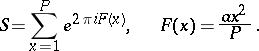 |
Gauss calculated the precise value of  :
:
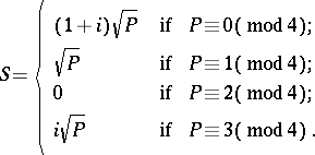 |
A whole series of independent articles applying trigonometric sums appeared at the beginning of the 20th century.
H. Weyl studied the distribution of the fractional parts of a polynomial
 |
with real coefficients  , and considered sums
  with a function
  of the form
  , where
  is a non-zero integer. I.M. Vinogradov (1917), in the study of the distribution of integer points in regions of the plane and in space, considered sums
  with a function
  of which it was required only that its second derivative satisfy the conditions
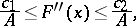 |
where  are absolute positive constants and
  . G.H. Hardy and J.E. Littlewood (1918), having obtained an approximate functional equation of the Riemann zeta-function, considered the sum
  with a function
  of the form
 |
where  is a real parameter,
  .
.
In all these papers it was required to find a best possible bound of the modulus of the sum  .
.
The general scheme for studying these problems in number theory by the method of trigonometric sums is as follows. One writes down the exact formula expressing the number of solutions of the equation under study, or the number of fractional parts of the function under study occurring in a given interval, or the number of integer points in a given region, in the form of an integral of trigonometric sums or in the form of a series whose coefficients are trigonometric sums. The exact formula is expressed as the sum of two terms, the principal and the secondary term (e.g. if one is considering the Fourier series of the characteristic function of an interval, then the principal term is obtained from the zero coefficient of the Fourier series); the principal term supplies the principal term of the asymptotic formula, the secondary term supplies the remainder term. In additive problems such as the Waring problem, the Goldbach problem, etc., the principal term is studied by a method close to the circle method of Hardy–Littlewood–Ramanujan (this method is called the circle method in the form of Vinogradov trigonometric sums). In the majority of other problems (the distribution of fractional parts, integer points in regions, etc.), the principal term is obtained trivially. There now arises the problem of estimating the remainder term, and if it can be proved that it is a quantity of smaller order than the principal term, then the asymptotic formula has been proved.
The main problem in estimating the remainder term is the problem of whether more precise estimates of trigonometric sums are possible. Concerning methods of estimating trigonometric sums, see Trigonometric sum, and also Vinogradov method; Waring problem; Goldbach problem; Additive problems.
For references see Trigonometric sum.
Trigonometric sums, method of. Encyclopedia of Mathematics. URL: http://encyclopediaofmath.org/index.php?title=Trigonometric_sums,_method_of&oldid=49039