Difference between revisions of "Stable distribution"
Ulf Rehmann (talk | contribs) m (tex encoded by computer) |
Ulf Rehmann (talk | contribs) m (Undo revision 48797 by Ulf Rehmann (talk)) Tag: Undo |
||
| Line 1: | Line 1: | ||
| − | |||
| − | |||
| − | |||
| − | |||
| − | |||
| − | |||
| − | |||
| − | |||
| − | |||
| − | |||
| − | |||
| − | |||
{{MSC|60E07}} | {{MSC|60E07}} | ||
[[Category:Distribution theory]] | [[Category:Distribution theory]] | ||
| − | A probability distribution with the property that for any | + | A probability distribution with the property that for any <img align="absmiddle" border="0" src="https://www.encyclopediaofmath.org/legacyimages/s/s087/s087110/s0871101.png" />, <img align="absmiddle" border="0" src="https://www.encyclopediaofmath.org/legacyimages/s/s087/s087110/s0871102.png" />, <img align="absmiddle" border="0" src="https://www.encyclopediaofmath.org/legacyimages/s/s087/s087110/s0871103.png" />, <img align="absmiddle" border="0" src="https://www.encyclopediaofmath.org/legacyimages/s/s087/s087110/s0871104.png" />, the relation |
| − | |||
| − | |||
| − | |||
| − | the relation | ||
| − | + | <table class="eq" style="width:100%;"> <tr><td valign="top" style="width:94%;text-align:center;"><img align="absmiddle" border="0" src="https://www.encyclopediaofmath.org/legacyimages/s/s087/s087110/s0871105.png" /></td> <td valign="top" style="width:5%;text-align:right;">(1)</td></tr></table> | |
| − | |||
| − | |||
| − | |||
| − | |||
| − | holds, where | + | holds, where <img align="absmiddle" border="0" src="https://www.encyclopediaofmath.org/legacyimages/s/s087/s087110/s0871106.png" /> and <img align="absmiddle" border="0" src="https://www.encyclopediaofmath.org/legacyimages/s/s087/s087110/s0871107.png" /> is a certain constant, <img align="absmiddle" border="0" src="https://www.encyclopediaofmath.org/legacyimages/s/s087/s087110/s0871108.png" /> is the distribution function of the stable distribution and <img align="absmiddle" border="0" src="https://www.encyclopediaofmath.org/legacyimages/s/s087/s087110/s0871109.png" /> is the convolution operator for two distribution functions. |
| − | |||
| − | is a certain constant, | ||
| − | is the distribution function of the stable distribution and | ||
| − | is the convolution operator for two distribution functions. | ||
The characteristic function of a stable distribution is of the form | The characteristic function of a stable distribution is of the form | ||
| − | + | <table class="eq" style="width:100%;"> <tr><td valign="top" style="width:94%;text-align:center;"><img align="absmiddle" border="0" src="https://www.encyclopediaofmath.org/legacyimages/s/s087/s087110/s08711010.png" /></td> <td valign="top" style="width:5%;text-align:right;">(2)</td></tr></table> | |
| − | |||
| − | |||
| − | |||
| − | |||
| − | |||
| − | |||
| − | |||
| − | |||
| − | |||
| − | |||
| − | where | + | where <img align="absmiddle" border="0" src="https://www.encyclopediaofmath.org/legacyimages/s/s087/s087110/s08711011.png" />, <img align="absmiddle" border="0" src="https://www.encyclopediaofmath.org/legacyimages/s/s087/s087110/s08711012.png" />, <img align="absmiddle" border="0" src="https://www.encyclopediaofmath.org/legacyimages/s/s087/s087110/s08711013.png" />, <img align="absmiddle" border="0" src="https://www.encyclopediaofmath.org/legacyimages/s/s087/s087110/s08711014.png" /> is any real number, and |
| − | |||
| − | |||
| − | |||
| − | is any real number, and | ||
| − | + | <table class="eq" style="width:100%;"> <tr><td valign="top" style="width:94%;text-align:center;"><img align="absmiddle" border="0" src="https://www.encyclopediaofmath.org/legacyimages/s/s087/s087110/s08711015.png" /></td> </tr></table> | |
| − | |||
| − | |||
| − | The number | + | The number <img align="absmiddle" border="0" src="https://www.encyclopediaofmath.org/legacyimages/s/s087/s087110/s08711016.png" /> is called the exponent of the stable distribution. A stable distribution with exponent <img align="absmiddle" border="0" src="https://www.encyclopediaofmath.org/legacyimages/s/s087/s087110/s08711017.png" /> is a [[Normal distribution|normal distribution]], an example of a stable distribution with exponent <img align="absmiddle" border="0" src="https://www.encyclopediaofmath.org/legacyimages/s/s087/s087110/s08711018.png" /> is the [[Cauchy distribution|Cauchy distribution]], a stable distribution which is a [[Degenerate distribution|degenerate distribution]] on the line. A stable distribution is an [[Infinitely-divisible distribution|infinitely-divisible distribution]]; for stable distributions with exponent <img align="absmiddle" border="0" src="https://www.encyclopediaofmath.org/legacyimages/s/s087/s087110/s08711019.png" />, <img align="absmiddle" border="0" src="https://www.encyclopediaofmath.org/legacyimages/s/s087/s087110/s08711020.png" />, one has the [[Lévy canonical representation|Lévy canonical representation]] with characteristic <img align="absmiddle" border="0" src="https://www.encyclopediaofmath.org/legacyimages/s/s087/s087110/s08711021.png" />, |
| − | is called the exponent of the stable distribution. A stable distribution with exponent | ||
| − | is a [[Normal distribution|normal distribution]], an example of a stable distribution with exponent | ||
| − | is the [[Cauchy distribution|Cauchy distribution]], a stable distribution which is a [[Degenerate distribution|degenerate distribution]] on the line. A stable distribution is an [[Infinitely-divisible distribution|infinitely-divisible distribution]]; for stable distributions with exponent | ||
| − | |||
| − | one has the [[Lévy canonical representation|Lévy canonical representation]] with characteristic | ||
| − | + | <table class="eq" style="width:100%;"> <tr><td valign="top" style="width:94%;text-align:center;"><img align="absmiddle" border="0" src="https://www.encyclopediaofmath.org/legacyimages/s/s087/s087110/s08711022.png" /></td> </tr></table> | |
| − | |||
| − | |||
| − | |||
| − | |||
| − | |||
| − | |||
| − | |||
| − | + | <table class="eq" style="width:100%;"> <tr><td valign="top" style="width:94%;text-align:center;"><img align="absmiddle" border="0" src="https://www.encyclopediaofmath.org/legacyimages/s/s087/s087110/s08711023.png" /></td> </tr></table> | |
| − | |||
| − | |||
| − | where | + | where <img align="absmiddle" border="0" src="https://www.encyclopediaofmath.org/legacyimages/s/s087/s087110/s08711024.png" /> is any real number. |
| − | is any real number. | ||
| − | A stable distribution, excluding the degenerate case, possesses a density. This density is infinitely differentiable, unimodal and different from zero either on the whole line or on a half-line. For a stable distribution with exponent | + | A stable distribution, excluding the degenerate case, possesses a density. This density is infinitely differentiable, unimodal and different from zero either on the whole line or on a half-line. For a stable distribution with exponent <img align="absmiddle" border="0" src="https://www.encyclopediaofmath.org/legacyimages/s/s087/s087110/s08711025.png" />, <img align="absmiddle" border="0" src="https://www.encyclopediaofmath.org/legacyimages/s/s087/s087110/s08711026.png" />, one has the relations |
| − | |||
| − | one has the relations | ||
| − | + | <table class="eq" style="width:100%;"> <tr><td valign="top" style="width:94%;text-align:center;"><img align="absmiddle" border="0" src="https://www.encyclopediaofmath.org/legacyimages/s/s087/s087110/s08711027.png" /></td> </tr></table> | |
| − | |||
| − | |||
| − | |||
| − | |||
| − | |||
| − | for | + | for <img align="absmiddle" border="0" src="https://www.encyclopediaofmath.org/legacyimages/s/s087/s087110/s08711028.png" />, where <img align="absmiddle" border="0" src="https://www.encyclopediaofmath.org/legacyimages/s/s087/s087110/s08711029.png" /> is the density of the stable distribution. An explicit form of the density of a stable distribution is known only in a few cases. One of the basic problems in the theory of stable distributions is the description of their domains of attraction (cf. [[Attraction domain of a stable distribution|Attraction domain of a stable distribution]]). |
| − | where | ||
| − | is the density of the stable distribution. An explicit form of the density of a stable distribution is known only in a few cases. One of the basic problems in the theory of stable distributions is the description of their domains of attraction (cf. [[Attraction domain of a stable distribution|Attraction domain of a stable distribution]]). | ||
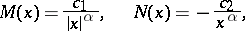
| − | In the set of stable distributions one singles out the set of strictly-stable distributions, for which equation (1) holds with | + | In the set of stable distributions one singles out the set of strictly-stable distributions, for which equation (1) holds with <img align="absmiddle" border="0" src="https://www.encyclopediaofmath.org/legacyimages/s/s087/s087110/s08711030.png" />. The characteristic function of a strictly-stable distribution with exponent <img align="absmiddle" border="0" src="https://www.encyclopediaofmath.org/legacyimages/s/s087/s087110/s08711031.png" /> (<img align="absmiddle" border="0" src="https://www.encyclopediaofmath.org/legacyimages/s/s087/s087110/s08711032.png" />) is given by formula (2) with <img align="absmiddle" border="0" src="https://www.encyclopediaofmath.org/legacyimages/s/s087/s087110/s08711033.png" />. For <img align="absmiddle" border="0" src="https://www.encyclopediaofmath.org/legacyimages/s/s087/s087110/s08711034.png" /> a strictly-stable distribution can only be a Cauchy distribution. Spectrally-positive (negative) stable distributions are characterized by the fact that in their Lévy canonical representation <img align="absmiddle" border="0" src="https://www.encyclopediaofmath.org/legacyimages/s/s087/s087110/s08711035.png" /> (<img align="absmiddle" border="0" src="https://www.encyclopediaofmath.org/legacyimages/s/s087/s087110/s08711036.png" />). The Laplace transform of a spectrally-positive stable distribution exists if <img align="absmiddle" border="0" src="https://www.encyclopediaofmath.org/legacyimages/s/s087/s087110/s08711037.png" />: |
| − | The characteristic function of a strictly-stable distribution with exponent | ||
| − | |||
| − | is given by formula (2) with | ||
| − | For | ||
| − | a strictly-stable distribution can only be a Cauchy distribution. Spectrally-positive (negative) stable distributions are characterized by the fact that in their Lévy canonical representation | ||
| − | |||
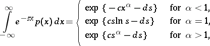
| − | The Laplace transform of a spectrally-positive stable distribution exists if | ||
| − | + | <table class="eq" style="width:100%;"> <tr><td valign="top" style="width:94%;text-align:center;"><img align="absmiddle" border="0" src="https://www.encyclopediaofmath.org/legacyimages/s/s087/s087110/s08711038.png" /></td> </tr></table> | |
| − | |||
| − | |||
| − | where | + | where <img align="absmiddle" border="0" src="https://www.encyclopediaofmath.org/legacyimages/s/s087/s087110/s08711039.png" /> is the density of the spectrally-positive stable distribution with exponent <img align="absmiddle" border="0" src="https://www.encyclopediaofmath.org/legacyimages/s/s087/s087110/s08711040.png" />, <img align="absmiddle" border="0" src="https://www.encyclopediaofmath.org/legacyimages/s/s087/s087110/s08711041.png" />, <img align="absmiddle" border="0" src="https://www.encyclopediaofmath.org/legacyimages/s/s087/s087110/s08711042.png" />, <img align="absmiddle" border="0" src="https://www.encyclopediaofmath.org/legacyimages/s/s087/s087110/s08711043.png" /> is a real number, and those branches of the many-valued functions <img align="absmiddle" border="0" src="https://www.encyclopediaofmath.org/legacyimages/s/s087/s087110/s08711044.png" />, <img align="absmiddle" border="0" src="https://www.encyclopediaofmath.org/legacyimages/s/s087/s087110/s08711045.png" /> are chosen for which <img align="absmiddle" border="0" src="https://www.encyclopediaofmath.org/legacyimages/s/s087/s087110/s08711046.png" /> is real and <img align="absmiddle" border="0" src="https://www.encyclopediaofmath.org/legacyimages/s/s087/s087110/s08711047.png" /> for <img align="absmiddle" border="0" src="https://www.encyclopediaofmath.org/legacyimages/s/s087/s087110/s08711048.png" />. |
| − | is the density of the spectrally-positive stable distribution with exponent | ||
| − | |||
| − | |||
| − | |||
| − | is a real number, and those branches of the many-valued functions | ||
| − | |||
| − | are chosen for which | ||
| − | is real and | ||
| − | |||
| − | Stable distributions, like infinitely-divisible distributions, correspond to stationary stochastic processes with stationary independent increments. A stochastically-continuous stationary stochastic process with independent increments | + | Stable distributions, like infinitely-divisible distributions, correspond to stationary stochastic processes with stationary independent increments. A stochastically-continuous stationary stochastic process with independent increments <img align="absmiddle" border="0" src="https://www.encyclopediaofmath.org/legacyimages/s/s087/s087110/s08711049.png" /> is called stable if the increment <img align="absmiddle" border="0" src="https://www.encyclopediaofmath.org/legacyimages/s/s087/s087110/s08711050.png" /> has a stable distribution. |
| − | is called stable if the increment | ||
| − | has a stable distribution. | ||
====References==== | ====References==== | ||
Revision as of 14:53, 7 June 2020
2020 Mathematics Subject Classification: Primary: 60E07 [MSN][ZBL]
A probability distribution with the property that for any  ,
,  ,
,  ,
,  , the relation
 | (1) |
holds, where  and
and  is a certain constant,
  is the distribution function of the stable distribution and
  is the convolution operator for two distribution functions.
The characteristic function of a stable distribution is of the form
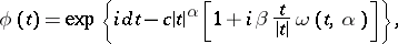 | (2) |
where  ,
,  ,
,  ,
,  is any real number, and
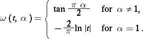 |
The number  is called the exponent of the stable distribution. A stable distribution with exponent
  is a normal distribution, an example of a stable distribution with exponent
  is the Cauchy distribution, a stable distribution which is a degenerate distribution on the line. A stable distribution is an infinitely-divisible distribution; for stable distributions with exponent
  ,
,  , one has the Lévy canonical representation with characteristic
  ,
,
 |
 |
where  is any real number.
A stable distribution, excluding the degenerate case, possesses a density. This density is infinitely differentiable, unimodal and different from zero either on the whole line or on a half-line. For a stable distribution with exponent  ,
,  , one has the relations
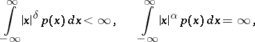 |
for  , where
  is the density of the stable distribution. An explicit form of the density of a stable distribution is known only in a few cases. One of the basic problems in the theory of stable distributions is the description of their domains of attraction (cf. Attraction domain of a stable distribution).
In the set of stable distributions one singles out the set of strictly-stable distributions, for which equation (1) holds with  . The characteristic function of a strictly-stable distribution with exponent
  (
( ) is given by formula (2) with
  . For
. For  a strictly-stable distribution can only be a Cauchy distribution. Spectrally-positive (negative) stable distributions are characterized by the fact that in their Lévy canonical representation
  (
( ). The Laplace transform of a spectrally-positive stable distribution exists if
  :
:
 |
where  is the density of the spectrally-positive stable distribution with exponent
  ,
,  ,
,  ,
,  is a real number, and those branches of the many-valued functions
  ,
,  are chosen for which
  is real and
  for
for  .
.
Stable distributions, like infinitely-divisible distributions, correspond to stationary stochastic processes with stationary independent increments. A stochastically-continuous stationary stochastic process with independent increments  is called stable if the increment
  has a stable distribution.
References
| [GK] | B.V. Gnedenko, A.N. Kolmogorov, "Limit distributions for sums of independent random variables" , Addison-Wesley (1954) (Translated from Russian) MR0062975 Zbl 0056.36001 |
| [PR] | Yu.V. Prohorov, Yu.A. Rozanov, "Probability theory, basic concepts. Limit theorems, random processes" , Springer (1969) (Translated from Russian) MR0251754 |
| [IL] | I.A. Ibragimov, Yu.V. Linnik, "Independent and stationary sequences of random variables" , Wolters-Noordhoff (1971) (Translated from Russian) MR0322926 Zbl 0219.60027 |
| [S] | A.V. Skorohod, "Stochastic processes with independent increments" , Kluwer (1991) (Translated from Russian) MR0094842 |
| [Z] | V.M. Zolotarev, "One-dimensional stable distributions" , Amer. Math. Soc. (1986) (Translated from Russian) MR0854867 Zbl 0589.60015 |
Comments
In practically all the literature the characteristic function of the stable distributions contains an error of sign; for the correct formulas see [H].
References
| [H] | P. Hall, "A comedy of errors: the canonical term for the stable characteristic functions" Bull. London Math. Soc. , 13 (1981) pp. 23–27 |
Stable distribution. Encyclopedia of Mathematics. URL: http://encyclopediaofmath.org/index.php?title=Stable_distribution&oldid=49441