Difference between revisions of "Spherical harmonics, method of"
Ulf Rehmann (talk | contribs) m (tex encoded by computer) |
Ulf Rehmann (talk | contribs) m (Undo revision 48776 by Ulf Rehmann (talk)) Tag: Undo |
||
| Line 1: | Line 1: | ||
| − | |||
| − | |||
| − | |||
| − | |||
| − | |||
| − | |||
| − | |||
| − | |||
| − | |||
| − | |||
| − | |||
| − | |||
A method for obtaining an approximate solution of a kinetic equation by the decomposition of the phase density of the particles into a finite sum of [[Spherical functions|spherical functions]] in arguments that define the direction of the velocity of the particles (see [[#References|[1]]]). The method is widely used in the solution of problems of neutron physics. | A method for obtaining an approximate solution of a kinetic equation by the decomposition of the phase density of the particles into a finite sum of [[Spherical functions|spherical functions]] in arguments that define the direction of the velocity of the particles (see [[#References|[1]]]). The method is widely used in the solution of problems of neutron physics. | ||
In one-dimensional plane geometry the stationary, integro-differential, kinetic transport equation (given an isotropic scattering of the particles) | In one-dimensional plane geometry the stationary, integro-differential, kinetic transport equation (given an isotropic scattering of the particles) | ||
| − | + | <table class="eq" style="width:100%;"> <tr><td valign="top" style="width:94%;text-align:center;"><img align="absmiddle" border="0" src="https://www.encyclopediaofmath.org/legacyimages/s/s086/s086700/s0867001.png" /></td> <td valign="top" style="width:5%;text-align:right;">(1)</td></tr></table> | |
| − | |||
| − | |||
| − | |||
| − | |||
| − | |||
| − | |||
| − | |||
| − | is replaced by an approximate system of differential equations for | + | is replaced by an approximate system of differential equations for <img align="absmiddle" border="0" src="https://www.encyclopediaofmath.org/legacyimages/s/s086/s086700/s0867002.png" /> — the approximate values of the Fourier coefficients |
| − | the approximate values of the Fourier coefficients | ||
| − | + | <table class="eq" style="width:100%;"> <tr><td valign="top" style="width:94%;text-align:center;"><img align="absmiddle" border="0" src="https://www.encyclopediaofmath.org/legacyimages/s/s086/s086700/s0867003.png" /></td> <td valign="top" style="width:5%;text-align:right;">(2)</td></tr></table> | |
| − | |||
| − | |||
| − | |||
A system of the form | A system of the form | ||
| − | + | <table class="eq" style="width:100%;"> <tr><td valign="top" style="width:94%;text-align:center;"><img align="absmiddle" border="0" src="https://www.encyclopediaofmath.org/legacyimages/s/s086/s086700/s0867004.png" /></td> <td valign="top" style="width:5%;text-align:right;">(3)</td></tr></table> | |
| − | |||
| − | |||
| − | |||
| − | |||
| − | |||
| − | |||
arises, under the condition | arises, under the condition | ||
| − | + | <table class="eq" style="width:100%;"> <tr><td valign="top" style="width:94%;text-align:center;"><img align="absmiddle" border="0" src="https://www.encyclopediaofmath.org/legacyimages/s/s086/s086700/s0867005.png" /></td> <td valign="top" style="width:5%;text-align:right;">(4)</td></tr></table> | |
| − | |||
| − | |||
| − | Here, | + | Here, <img align="absmiddle" border="0" src="https://www.encyclopediaofmath.org/legacyimages/s/s086/s086700/s0867006.png" /> is the phase density of the particles that are scattered in the matter, <img align="absmiddle" border="0" src="https://www.encyclopediaofmath.org/legacyimages/s/s086/s086700/s0867007.png" /> is the average number of secondary particles arising from one act of interaction with the particles of matter, and <img align="absmiddle" border="0" src="https://www.encyclopediaofmath.org/legacyimages/s/s086/s086700/s0867008.png" /> is the Legendre polynomial of degree <img align="absmiddle" border="0" src="https://www.encyclopediaofmath.org/legacyimages/s/s086/s086700/s0867009.png" /> (cf. [[Legendre polynomials|Legendre polynomials]]). System (3) defines the <img align="absmiddle" border="0" src="https://www.encyclopediaofmath.org/legacyimages/s/s086/s086700/s08670010.png" />-approximation of the method of spherical harmonics for equation (1). The approximate value of the phase density is |
| − | is the phase density of the particles that are scattered in the matter, | ||
| − | is the average number of secondary particles arising from one act of interaction with the particles of matter, and | ||
| − | is the Legendre polynomial of degree | ||
| − | cf. [[Legendre polynomials|Legendre polynomials]]). System (3) defines the | ||
| − | approximation of the method of spherical harmonics for equation (1). The approximate value of the phase density is | ||
| − | + | <table class="eq" style="width:100%;"> <tr><td valign="top" style="width:94%;text-align:center;"><img align="absmiddle" border="0" src="https://www.encyclopediaofmath.org/legacyimages/s/s086/s086700/s08670011.png" /></td> <td valign="top" style="width:5%;text-align:right;">(5)</td></tr></table> | |
| − | |||
| − | |||
| − | |||
| − | |||
| − | |||
For equation (1), the typical boundary conditions take the form | For equation (1), the typical boundary conditions take the form | ||
| − | + | <table class="eq" style="width:100%;"> <tr><td valign="top" style="width:94%;text-align:center;"><img align="absmiddle" border="0" src="https://www.encyclopediaofmath.org/legacyimages/s/s086/s086700/s08670012.png" /></td> <td valign="top" style="width:5%;text-align:right;">(6)</td></tr></table> | |
| − | |||
| − | Boundary conditions of this type exist in, for example, the problem in neutron physics of the critical conditions of a layer of thickness | + | Boundary conditions of this type exist in, for example, the problem in neutron physics of the critical conditions of a layer of thickness <img align="absmiddle" border="0" src="https://www.encyclopediaofmath.org/legacyimages/s/s086/s086700/s08670013.png" /> with free surfaces <img align="absmiddle" border="0" src="https://www.encyclopediaofmath.org/legacyimages/s/s086/s086700/s08670014.png" /> and <img align="absmiddle" border="0" src="https://www.encyclopediaofmath.org/legacyimages/s/s086/s086700/s08670015.png" /> (boundaries with vacuum). In this problem, a positive solution of (1) and (6), as well as the eigenvalue <img align="absmiddle" border="0" src="https://www.encyclopediaofmath.org/legacyimages/s/s086/s086700/s08670016.png" />, must be found. |
| − | with free surfaces | ||
| − | and | ||
| − | boundaries with vacuum). In this problem, a positive solution of (1) and (6), as well as the eigenvalue | ||
| − | must be found. | ||
In the method of spherical harmonics, it is natural to replace (6) by | In the method of spherical harmonics, it is natural to replace (6) by | ||
| − | + | <table class="eq" style="width:100%;"> <tr><td valign="top" style="width:94%;text-align:center;"><img align="absmiddle" border="0" src="https://www.encyclopediaofmath.org/legacyimages/s/s086/s086700/s08670017.png" /></td> <td valign="top" style="width:5%;text-align:right;">(7)</td></tr></table> | |
| − | |||
| − | However, this approach involves twice as many conditions than are required for a partial solution of (3). In practice, a different set of values has been tested in (7). The best result is obtained by conditions with | + | However, this approach involves twice as many conditions than are required for a partial solution of (3). In practice, a different set of values has been tested in (7). The best result is obtained by conditions with <img align="absmiddle" border="0" src="https://www.encyclopediaofmath.org/legacyimages/s/s086/s086700/s08670018.png" />, <img align="absmiddle" border="0" src="https://www.encyclopediaofmath.org/legacyimages/s/s086/s086700/s08670019.png" />. For the single-velocity transport equation of a general type, the [[Vladimirov variational principle|Vladimirov variational principle]] leads to a system of equations of the method of spherical harmonics and the given boundary conditions (when choosing the experimental functions in the form of a linear combination of [[Spherical harmonics|spherical harmonics]]). In three-dimensional geometry, the boundary conditions can be written in the form |
| − | |||
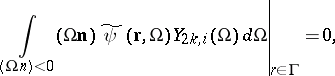
| − | For the single-velocity transport equation of a general type, the [[Vladimirov variational principle|Vladimirov variational principle]] leads to a system of equations of the method of spherical harmonics and the given boundary conditions (when choosing the experimental functions in the form of a linear combination of [[Spherical harmonics|spherical harmonics]]). In three-dimensional geometry, the boundary conditions can be written in the form | ||
| − | + | <table class="eq" style="width:100%;"> <tr><td valign="top" style="width:94%;text-align:center;"><img align="absmiddle" border="0" src="https://www.encyclopediaofmath.org/legacyimages/s/s086/s086700/s08670020.png" /></td> <td valign="top" style="width:5%;text-align:right;">(8)</td></tr></table> | |
| − | |||
| − | |||
| − | |||
| − | |||
| − | |||
| − | + | <table class="eq" style="width:100%;"> <tr><td valign="top" style="width:94%;text-align:center;"><img align="absmiddle" border="0" src="https://www.encyclopediaofmath.org/legacyimages/s/s086/s086700/s08670021.png" /></td> </tr></table> | |
| − | |||
| − | |||
| − | Here | + | Here <img align="absmiddle" border="0" src="https://www.encyclopediaofmath.org/legacyimages/s/s086/s086700/s08670022.png" /> is a vector of space coordinates, <img align="absmiddle" border="0" src="https://www.encyclopediaofmath.org/legacyimages/s/s086/s086700/s08670023.png" /> is a unit vector of the velocity of the particle with spherical coordinates <img align="absmiddle" border="0" src="https://www.encyclopediaofmath.org/legacyimages/s/s086/s086700/s08670024.png" />, <img align="absmiddle" border="0" src="https://www.encyclopediaofmath.org/legacyimages/s/s086/s086700/s08670025.png" /> is the unit vector of the exterior normal to the piecewise-smooth surface <img align="absmiddle" border="0" src="https://www.encyclopediaofmath.org/legacyimages/s/s086/s086700/s08670026.png" /> that bounds the convex domain in space in which the problem is solved, |
| − | is a vector of space coordinates, | ||
| − | is a unit vector of the velocity of the particle with spherical coordinates | ||
| − | |||
| − | is the unit vector of the exterior normal to the piecewise-smooth surface | ||
| − | that bounds the convex domain in space in which the problem is solved, | ||
| − | + | <table class="eq" style="width:100%;"> <tr><td valign="top" style="width:94%;text-align:center;"><img align="absmiddle" border="0" src="https://www.encyclopediaofmath.org/legacyimages/s/s086/s086700/s08670027.png" /></td> </tr></table> | |
| − | |||
| − | |||
| − | |||
| − | |||
| − | + | <table class="eq" style="width:100%;"> <tr><td valign="top" style="width:94%;text-align:center;"><img align="absmiddle" border="0" src="https://www.encyclopediaofmath.org/legacyimages/s/s086/s086700/s08670028.png" /></td> </tr></table> | |
| − | |||
| − | |||
| − | are the spherical functions, | + | are the spherical functions, <img align="absmiddle" border="0" src="https://www.encyclopediaofmath.org/legacyimages/s/s086/s086700/s08670029.png" /> are the associated Legendre functions of the first kind (<img align="absmiddle" border="0" src="https://www.encyclopediaofmath.org/legacyimages/s/s086/s086700/s08670030.png" /> are the Legendre polynomials). |
| − | are the associated Legendre functions of the first kind ( | ||
| − | are the Legendre polynomials). | ||
| − | The lowest approximations | + | The lowest approximations <img align="absmiddle" border="0" src="https://www.encyclopediaofmath.org/legacyimages/s/s086/s086700/s08670031.png" /> of the method of spherical harmonics are widely used in solving problems of neutron physics and give good results well away from the boundaries of the domain, sources and strong neutron absorbers. The theory of growth is also constructed in a <img align="absmiddle" border="0" src="https://www.encyclopediaofmath.org/legacyimages/s/s086/s086700/s08670032.png" />-approximation. The generalized solution of the method of spherical harmonics converges to the solution of the transport equation when <img align="absmiddle" border="0" src="https://www.encyclopediaofmath.org/legacyimages/s/s086/s086700/s08670033.png" /> (see [[#References|[2]]]). The rate of the convergence <img align="absmiddle" border="0" src="https://www.encyclopediaofmath.org/legacyimages/s/s086/s086700/s08670034.png" /> is easily estimated, by comparing the integral equations for <img align="absmiddle" border="0" src="https://www.encyclopediaofmath.org/legacyimages/s/s086/s086700/s08670035.png" /> and <img align="absmiddle" border="0" src="https://www.encyclopediaofmath.org/legacyimages/s/s086/s086700/s08670036.png" />, i.e. by estimating the proximity of their kernels. Equation (1) with the boundary conditions (6) reduces to an integral equation with the kernel |
| − | of the method of spherical harmonics are widely used in solving problems of neutron physics and give good results well away from the boundaries of the domain, sources and strong neutron absorbers. The theory of growth is also constructed in a | ||
| − | approximation. The generalized solution of the method of spherical harmonics converges to the solution of the transport equation when | ||
| − | see [[#References|[2]]]). The rate of the convergence | ||
| − | is easily estimated, by comparing the integral equations for | ||
| − | and | ||
| − | i.e. by estimating the proximity of their kernels. Equation (1) with the boundary conditions (6) reduces to an integral equation with the kernel | ||
| − | + | <table class="eq" style="width:100%;"> <tr><td valign="top" style="width:94%;text-align:center;"><img align="absmiddle" border="0" src="https://www.encyclopediaofmath.org/legacyimages/s/s086/s086700/s08670037.png" /></td> </tr></table> | |
| − | |||
| − | |||
| − | |||
| − | |||
System (3), given boundary conditions analogous to (6), | System (3), given boundary conditions analogous to (6), | ||
| − | + | <table class="eq" style="width:100%;"> <tr><td valign="top" style="width:94%;text-align:center;"><img align="absmiddle" border="0" src="https://www.encyclopediaofmath.org/legacyimages/s/s086/s086700/s08670038.png" /></td> <td valign="top" style="width:5%;text-align:right;">(9)</td></tr></table> | |
| − | |||
| − | |||
| − | |||
| − | |||
| − | |||
| − | + | where <img align="absmiddle" border="0" src="https://www.encyclopediaofmath.org/legacyimages/s/s086/s086700/s08670039.png" /> are the roots of <img align="absmiddle" border="0" src="https://www.encyclopediaofmath.org/legacyimages/s/s086/s086700/s08670040.png" />, reduces to an integral equation with kernel | |
| − | |||
| − | |||
| − | |||
| − | |||
| − | |||
| − | + | <table class="eq" style="width:100%;"> <tr><td valign="top" style="width:94%;text-align:center;"><img align="absmiddle" border="0" src="https://www.encyclopediaofmath.org/legacyimages/s/s086/s086700/s08670041.png" /></td> </tr></table> | |
| − | |||
| − | |||
| − | |||
| − | + | where <img align="absmiddle" border="0" src="https://www.encyclopediaofmath.org/legacyimages/s/s086/s086700/s08670042.png" /> are the weights of the [[Gauss quadrature formula|Gauss quadrature formula]] for the system of nodes <img align="absmiddle" border="0" src="https://www.encyclopediaofmath.org/legacyimages/s/s086/s086700/s08670043.png" />. The singularity of the function <img align="absmiddle" border="0" src="https://www.encyclopediaofmath.org/legacyimages/s/s086/s086700/s08670044.png" /> leads to a slow convergence for large <img align="absmiddle" border="0" src="https://www.encyclopediaofmath.org/legacyimages/s/s086/s086700/s08670045.png" />: | |
| − | |||
| − | |||
| − | + | <table class="eq" style="width:100%;"> <tr><td valign="top" style="width:94%;text-align:center;"><img align="absmiddle" border="0" src="https://www.encyclopediaofmath.org/legacyimages/s/s086/s086700/s08670046.png" /></td> </tr></table> | |
| − | |||
| − | |||
| − | |||
| − | |||
| − | The approximate eigenvalue converges to an exact eigenvalue at a rate of | + | The approximate eigenvalue converges to an exact eigenvalue at a rate of <img align="absmiddle" border="0" src="https://www.encyclopediaofmath.org/legacyimages/s/s086/s086700/s08670047.png" />. |
The boundary conditions (9) arise naturally in the solution of the kinetic equation by the method of discrete ordinates, which consists of replacing (1) by the approximate system | The boundary conditions (9) arise naturally in the solution of the kinetic equation by the method of discrete ordinates, which consists of replacing (1) by the approximate system | ||
| − | + | <table class="eq" style="width:100%;"> <tr><td valign="top" style="width:94%;text-align:center;"><img align="absmiddle" border="0" src="https://www.encyclopediaofmath.org/legacyimages/s/s086/s086700/s08670048.png" /></td> <td valign="top" style="width:5%;text-align:right;">(10)</td></tr></table> | |
| − | |||
| − | |||
| − | |||
| − | |||
| − | |||
| − | |||
| − | |||
The method of discrete ordinates in one-dimensional geometry is equivalent to the method of spherical harmonics (see [[#References|[3]]]), since the system (10) can be obtained from (3) by means of a linear transformation of the unknown functions: | The method of discrete ordinates in one-dimensional geometry is equivalent to the method of spherical harmonics (see [[#References|[3]]]), since the system (10) can be obtained from (3) by means of a linear transformation of the unknown functions: | ||
| − | + | <table class="eq" style="width:100%;"> <tr><td valign="top" style="width:94%;text-align:center;"><img align="absmiddle" border="0" src="https://www.encyclopediaofmath.org/legacyimages/s/s086/s086700/s08670049.png" /></td> </tr></table> | |
| − | |||
| − | |||
| − | |||
However, in multi-dimensional problems, the method of spherical harmonics in the lowest approximations is more accurate than the method of discrete ordinates. | However, in multi-dimensional problems, the method of spherical harmonics in the lowest approximations is more accurate than the method of discrete ordinates. | ||
| Line 183: | Line 75: | ||
====References==== | ====References==== | ||
<table><TR><TD valign="top">[1]</TD> <TD valign="top"> G.I. Marchuk, V.I. Lebedev, "Numerical methods in the theory of neutron transport" , Harwood (1986) (Translated from Russian)</TD></TR><TR><TD valign="top">[2]</TD> <TD valign="top"> U.M. Sultangazin, "Convergence of the method of spherical harmonics for the non-stationary transport equation" ''USSR Comp. Math. Math. Phys.'' , '''14''' : 1 (1974) pp. 165–176 ''Zh. Vychisl. Mat. i Mat. Fiz.'' , '''14''' : 1 (1974) pp. 166–178</TD></TR><TR><TD valign="top">[3]</TD> <TD valign="top"> R.D. Richtmeyer, K.W. Morton, "Difference methods for initial-value problems" , Wiley (Interscience) (1967)</TD></TR></table> | <table><TR><TD valign="top">[1]</TD> <TD valign="top"> G.I. Marchuk, V.I. Lebedev, "Numerical methods in the theory of neutron transport" , Harwood (1986) (Translated from Russian)</TD></TR><TR><TD valign="top">[2]</TD> <TD valign="top"> U.M. Sultangazin, "Convergence of the method of spherical harmonics for the non-stationary transport equation" ''USSR Comp. Math. Math. Phys.'' , '''14''' : 1 (1974) pp. 165–176 ''Zh. Vychisl. Mat. i Mat. Fiz.'' , '''14''' : 1 (1974) pp. 166–178</TD></TR><TR><TD valign="top">[3]</TD> <TD valign="top"> R.D. Richtmeyer, K.W. Morton, "Difference methods for initial-value problems" , Wiley (Interscience) (1967)</TD></TR></table> | ||
| + | |||
| + | |||
====Comments==== | ====Comments==== | ||
| + | |||
====References==== | ====References==== | ||
<table><TR><TD valign="top">[a1]</TD> <TD valign="top"> G.I. Marchuk, "Methods of numerical mathematics" , Springer (1975) (Translated from Russian)</TD></TR><TR><TD valign="top">[a2]</TD> <TD valign="top"> B. Davison, J.B. Sykes, "Neutron transport theory" , Clarendon Press (1957)</TD></TR><TR><TD valign="top">[a3]</TD> <TD valign="top"> K.M. Case, P.F. Zweifel, "Linear transport theory" , Addison-Wesley (1967)</TD></TR></table> | <table><TR><TD valign="top">[a1]</TD> <TD valign="top"> G.I. Marchuk, "Methods of numerical mathematics" , Springer (1975) (Translated from Russian)</TD></TR><TR><TD valign="top">[a2]</TD> <TD valign="top"> B. Davison, J.B. Sykes, "Neutron transport theory" , Clarendon Press (1957)</TD></TR><TR><TD valign="top">[a3]</TD> <TD valign="top"> K.M. Case, P.F. Zweifel, "Linear transport theory" , Addison-Wesley (1967)</TD></TR></table> | ||
Revision as of 14:53, 7 June 2020
A method for obtaining an approximate solution of a kinetic equation by the decomposition of the phase density of the particles into a finite sum of spherical functions in arguments that define the direction of the velocity of the particles (see [1]). The method is widely used in the solution of problems of neutron physics.
In one-dimensional plane geometry the stationary, integro-differential, kinetic transport equation (given an isotropic scattering of the particles)
 | (1) |
is replaced by an approximate system of differential equations for  — the approximate values of the Fourier coefficients
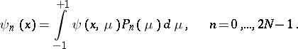 | (2) |
A system of the form
 | (3) |
arises, under the condition
 | (4) |
Here,  is the phase density of the particles that are scattered in the matter,
  is the average number of secondary particles arising from one act of interaction with the particles of matter, and
  is the Legendre polynomial of degree
  (cf. Legendre polynomials). System (3) defines the
  -approximation of the method of spherical harmonics for equation (1). The approximate value of the phase density is
 | (5) |
For equation (1), the typical boundary conditions take the form
 | (6) |
Boundary conditions of this type exist in, for example, the problem in neutron physics of the critical conditions of a layer of thickness  with free surfaces
  and
and  (boundaries with vacuum). In this problem, a positive solution of (1) and (6), as well as the eigenvalue
  , must be found.
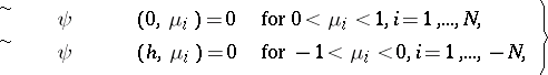
In the method of spherical harmonics, it is natural to replace (6) by
 | (7) |
However, this approach involves twice as many conditions than are required for a partial solution of (3). In practice, a different set of values has been tested in (7). The best result is obtained by conditions with  ,
,  . For the single-velocity transport equation of a general type, the Vladimirov variational principle leads to a system of equations of the method of spherical harmonics and the given boundary conditions (when choosing the experimental functions in the form of a linear combination of spherical harmonics). In three-dimensional geometry, the boundary conditions can be written in the form
 | (8) |
 |
Here  is a vector of space coordinates,
  is a unit vector of the velocity of the particle with spherical coordinates
  ,
,  is the unit vector of the exterior normal to the piecewise-smooth surface
  that bounds the convex domain in space in which the problem is solved,
 |
 |
are the spherical functions,  are the associated Legendre functions of the first kind (
 are the Legendre polynomials).
The lowest approximations  of the method of spherical harmonics are widely used in solving problems of neutron physics and give good results well away from the boundaries of the domain, sources and strong neutron absorbers. The theory of growth is also constructed in a
  -approximation. The generalized solution of the method of spherical harmonics converges to the solution of the transport equation when
  (see [2]). The rate of the convergence
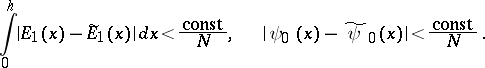
  is easily estimated, by comparing the integral equations for
  and
and  , i.e. by estimating the proximity of their kernels. Equation (1) with the boundary conditions (6) reduces to an integral equation with the kernel
 |
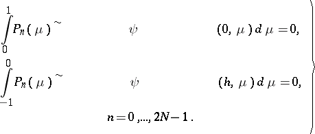
System (3), given boundary conditions analogous to (6),
 | (9) |
where  are the roots of
  , reduces to an integral equation with kernel
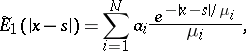 |
where  are the weights of the Gauss quadrature formula for the system of nodes
  . The singularity of the function
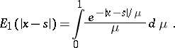
 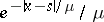 leads to a slow convergence for large
  :
:
 |
The approximate eigenvalue converges to an exact eigenvalue at a rate of  .
.
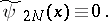
The boundary conditions (9) arise naturally in the solution of the kinetic equation by the method of discrete ordinates, which consists of replacing (1) by the approximate system
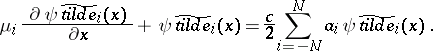 | (10) |
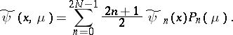
The method of discrete ordinates in one-dimensional geometry is equivalent to the method of spherical harmonics (see [3]), since the system (10) can be obtained from (3) by means of a linear transformation of the unknown functions:
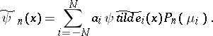 |
However, in multi-dimensional problems, the method of spherical harmonics in the lowest approximations is more accurate than the method of discrete ordinates.
References
| [1] | G.I. Marchuk, V.I. Lebedev, "Numerical methods in the theory of neutron transport" , Harwood (1986) (Translated from Russian) |
| [2] | U.M. Sultangazin, "Convergence of the method of spherical harmonics for the non-stationary transport equation" USSR Comp. Math. Math. Phys. , 14 : 1 (1974) pp. 165–176 Zh. Vychisl. Mat. i Mat. Fiz. , 14 : 1 (1974) pp. 166–178 |
| [3] | R.D. Richtmeyer, K.W. Morton, "Difference methods for initial-value problems" , Wiley (Interscience) (1967) |
Comments
References
| [a1] | G.I. Marchuk, "Methods of numerical mathematics" , Springer (1975) (Translated from Russian) |
| [a2] | B. Davison, J.B. Sykes, "Neutron transport theory" , Clarendon Press (1957) |
| [a3] | K.M. Case, P.F. Zweifel, "Linear transport theory" , Addison-Wesley (1967) |
Spherical harmonics, method of. Encyclopedia of Mathematics. URL: http://encyclopediaofmath.org/index.php?title=Spherical_harmonics,_method_of&oldid=48776