Difference between revisions of "Rao-Blackwell-Kolmogorov theorem"
Ulf Rehmann (talk | contribs) m (tex encoded by computer) |
Ulf Rehmann (talk | contribs) m (Undo revision 48437 by Ulf Rehmann (talk)) Tag: Undo |
||
| Line 1: | Line 1: | ||
| − | |||
| − | |||
| − | |||
| − | |||
| − | |||
| − | |||
| − | |||
| − | |||
| − | |||
| − | |||
| − | |||
| − | |||
A proposition from the theory of statistical estimation on which a method for the improvement of unbiased statistical estimators is based. | A proposition from the theory of statistical estimation on which a method for the improvement of unbiased statistical estimators is based. | ||
| − | Let | + | Let <img align="absmiddle" border="0" src="https://www.encyclopediaofmath.org/legacyimages/r/r077/r077550/r0775501.png" /> be a random variable with values in a sample space <img align="absmiddle" border="0" src="https://www.encyclopediaofmath.org/legacyimages/r/r077/r077550/r0775502.png" />, <img align="absmiddle" border="0" src="https://www.encyclopediaofmath.org/legacyimages/r/r077/r077550/r0775503.png" />, such that the family of probability distributions <img align="absmiddle" border="0" src="https://www.encyclopediaofmath.org/legacyimages/r/r077/r077550/r0775504.png" /> has a [[Sufficient statistic|sufficient statistic]] <img align="absmiddle" border="0" src="https://www.encyclopediaofmath.org/legacyimages/r/r077/r077550/r0775505.png" />, and let <img align="absmiddle" border="0" src="https://www.encyclopediaofmath.org/legacyimages/r/r077/r077550/r0775506.png" /> be a vector statistic with finite matrix of second moments. Then the mean <img align="absmiddle" border="0" src="https://www.encyclopediaofmath.org/legacyimages/r/r077/r077550/r0775507.png" /> of <img align="absmiddle" border="0" src="https://www.encyclopediaofmath.org/legacyimages/r/r077/r077550/r0775508.png" /> exists and, moreover, the conditional mean <img align="absmiddle" border="0" src="https://www.encyclopediaofmath.org/legacyimages/r/r077/r077550/r0775509.png" /> is an [[Unbiased estimator|unbiased estimator]] for <img align="absmiddle" border="0" src="https://www.encyclopediaofmath.org/legacyimages/r/r077/r077550/r07755010.png" />, that is, |
| − | be a random variable with values in a sample space | ||
| − | |||
| − | such that the family of probability distributions | ||
| − | has a [[Sufficient statistic|sufficient statistic]] | ||
| − | and let | ||
| − | be a vector statistic with finite matrix of second moments. Then the mean | ||
| − | of | ||
| − | exists and, moreover, the conditional mean | ||
| − | is an [[Unbiased estimator|unbiased estimator]] for | ||
| − | that is, | ||
| − | + | <table class="eq" style="width:100%;"> <tr><td valign="top" style="width:94%;text-align:center;"><img align="absmiddle" border="0" src="https://www.encyclopediaofmath.org/legacyimages/r/r077/r077550/r07755011.png" /></td> </tr></table> | |
| − | |||
| − | |||
| − | |||
| − | |||
| − | The Rao–Blackwell–Kolmogorov theorem states that under these conditions the quadratic risk of | + | The Rao–Blackwell–Kolmogorov theorem states that under these conditions the quadratic risk of <img align="absmiddle" border="0" src="https://www.encyclopediaofmath.org/legacyimages/r/r077/r077550/r07755012.png" /> does not exceed the quadratic risk of <img align="absmiddle" border="0" src="https://www.encyclopediaofmath.org/legacyimages/r/r077/r077550/r07755013.png" />, uniformly in <img align="absmiddle" border="0" src="https://www.encyclopediaofmath.org/legacyimages/r/r077/r077550/r07755014.png" />, i.e. for any vector <img align="absmiddle" border="0" src="https://www.encyclopediaofmath.org/legacyimages/r/r077/r077550/r07755015.png" /> of the same dimension as <img align="absmiddle" border="0" src="https://www.encyclopediaofmath.org/legacyimages/r/r077/r077550/r07755016.png" />, the inequality |
| − | does not exceed the quadratic risk of | ||
| − | uniformly in | ||
| − | i.e. for any vector | ||
| − | of the same dimension as | ||
| − | the inequality | ||
| − | + | <table class="eq" style="width:100%;"> <tr><td valign="top" style="width:94%;text-align:center;"><img align="absmiddle" border="0" src="https://www.encyclopediaofmath.org/legacyimages/r/r077/r077550/r07755017.png" /></td> </tr></table> | |
| − | |||
| − | |||
| − | |||
| − | + | <table class="eq" style="width:100%;"> <tr><td valign="top" style="width:94%;text-align:center;"><img align="absmiddle" border="0" src="https://www.encyclopediaofmath.org/legacyimages/r/r077/r077550/r07755018.png" /></td> </tr></table> | |
| − | |||
| − | |||
| − | |||
| − | |||
| − | holds for any | + | holds for any <img align="absmiddle" border="0" src="https://www.encyclopediaofmath.org/legacyimages/r/r077/r077550/r07755019.png" />. In particular, if <img align="absmiddle" border="0" src="https://www.encyclopediaofmath.org/legacyimages/r/r077/r077550/r07755020.png" /> is a one-dimensional statistic, then for any <img align="absmiddle" border="0" src="https://www.encyclopediaofmath.org/legacyimages/r/r077/r077550/r07755021.png" /> the variance <img align="absmiddle" border="0" src="https://www.encyclopediaofmath.org/legacyimages/r/r077/r077550/r07755022.png" /> of <img align="absmiddle" border="0" src="https://www.encyclopediaofmath.org/legacyimages/r/r077/r077550/r07755023.png" /> does not exceed the variance <img align="absmiddle" border="0" src="https://www.encyclopediaofmath.org/legacyimages/r/r077/r077550/r07755024.png" /> of <img align="absmiddle" border="0" src="https://www.encyclopediaofmath.org/legacyimages/r/r077/r077550/r07755025.png" />. |
| − | In particular, if | ||
| − | is a one-dimensional statistic, then for any | ||
| − | the variance | ||
| − | of | ||
| − | does not exceed the variance | ||
| − | of | ||
In the most general situation the Rao–Blackwell–Kolmogorov theorem states that averaging over a sufficient statistic does not lead to an increase of the risk with respect to any convex loss function. This implies that good statistical estimators should be looked for only in terms of sufficient statistics, that is, in the class of functions of sufficient statistics. | In the most general situation the Rao–Blackwell–Kolmogorov theorem states that averaging over a sufficient statistic does not lead to an increase of the risk with respect to any convex loss function. This implies that good statistical estimators should be looked for only in terms of sufficient statistics, that is, in the class of functions of sufficient statistics. | ||
| − | In case the family | + | In case the family <img align="absmiddle" border="0" src="https://www.encyclopediaofmath.org/legacyimages/r/r077/r077550/r07755026.png" /> is complete, that is, when the function of <img align="absmiddle" border="0" src="https://www.encyclopediaofmath.org/legacyimages/r/r077/r077550/r07755027.png" /> that is almost-everywhere equal to zero is the only unbiased estimator based on <img align="absmiddle" border="0" src="https://www.encyclopediaofmath.org/legacyimages/r/r077/r077550/r07755028.png" /> for zero, the unbiased estimator with uniformly minimal risk provided by the Rao–Blackwell–Kolmogorov theorem is unique. Thus, the Rao–Blackwell–Kolmogorov theorem gives a recipe for constructing best unbiased estimators: one has to take some unbiased estimator and then average it over a sufficient statistic. That is how the best unbiased estimator for the distribution function of the normal law is constructed in the following example, which is due to A.N. Kolmogorov. |
| − | is complete, that is, when the function of | ||
| − | that is almost-everywhere equal to zero is the only unbiased estimator based on | ||
| − | for zero, the unbiased estimator with uniformly minimal risk provided by the Rao–Blackwell–Kolmogorov theorem is unique. Thus, the Rao–Blackwell–Kolmogorov theorem gives a recipe for constructing best unbiased estimators: one has to take some unbiased estimator and then average it over a sufficient statistic. That is how the best unbiased estimator for the distribution function of the normal law is constructed in the following example, which is due to A.N. Kolmogorov. | ||
| − | |||
| − | |||
| − | |||
| − | |||
| − | |||
| − | |||
| − | |||
| − | |||
| − | |||
| − | |||
| − | |||
| − | |||
| − | |||
| − | |||
| − | + | Example. Given a realization of a random vector <img align="absmiddle" border="0" src="https://www.encyclopediaofmath.org/legacyimages/r/r077/r077550/r07755029.png" /> whose components <img align="absmiddle" border="0" src="https://www.encyclopediaofmath.org/legacyimages/r/r077/r077550/r07755030.png" />, <img align="absmiddle" border="0" src="https://www.encyclopediaofmath.org/legacyimages/r/r077/r077550/r07755031.png" />, <img align="absmiddle" border="0" src="https://www.encyclopediaofmath.org/legacyimages/r/r077/r077550/r07755032.png" />, are independent random variables subject to the same normal law <img align="absmiddle" border="0" src="https://www.encyclopediaofmath.org/legacyimages/r/r077/r077550/r07755033.png" />, it is required to estimate the distribution function | |
| − | |||
| − | |||
| − | |||
| − | |||
| − | + | <table class="eq" style="width:100%;"> <tr><td valign="top" style="width:94%;text-align:center;"><img align="absmiddle" border="0" src="https://www.encyclopediaofmath.org/legacyimages/r/r077/r077550/r07755034.png" /></td> </tr></table> | |
| − | |||
| − | |||
| − | + | The parameters <img align="absmiddle" border="0" src="https://www.encyclopediaofmath.org/legacyimages/r/r077/r077550/r07755035.png" /> and <img align="absmiddle" border="0" src="https://www.encyclopediaofmath.org/legacyimages/r/r077/r077550/r07755036.png" /> are supposed to be unknown. Since the family | |
| − | |||
| − | |||
| − | |||
| − | |||
| − | |||
| − | + | <table class="eq" style="width:100%;"> <tr><td valign="top" style="width:94%;text-align:center;"><img align="absmiddle" border="0" src="https://www.encyclopediaofmath.org/legacyimages/r/r077/r077550/r07755037.png" /></td> </tr></table> | |
| − | |||
| − | + | of normal laws has a complete sufficient statistic <img align="absmiddle" border="0" src="https://www.encyclopediaofmath.org/legacyimages/r/r077/r077550/r07755038.png" />, where | |
| − | |||
| − | |||
| − | + | <table class="eq" style="width:100%;"> <tr><td valign="top" style="width:94%;text-align:center;"><img align="absmiddle" border="0" src="https://www.encyclopediaofmath.org/legacyimages/r/r077/r077550/r07755039.png" /></td> </tr></table> | |
and | and | ||
| − | + | <table class="eq" style="width:100%;"> <tr><td valign="top" style="width:94%;text-align:center;"><img align="absmiddle" border="0" src="https://www.encyclopediaofmath.org/legacyimages/r/r077/r077550/r07755040.png" /></td> </tr></table> | |
| − | |||
| − | |||
| − | |||
| − | |||
| − | the Rao–Blackwell–Kolmogorov theorem can be used for the construction of the best unbiased estimator for the distribution function | + | the Rao–Blackwell–Kolmogorov theorem can be used for the construction of the best unbiased estimator for the distribution function <img align="absmiddle" border="0" src="https://www.encyclopediaofmath.org/legacyimages/r/r077/r077550/r07755041.png" />. As an initial statistic <img align="absmiddle" border="0" src="https://www.encyclopediaofmath.org/legacyimages/r/r077/r077550/r07755042.png" /> one may use, e.g., the empirical distribution function constructed from an arbitrary component <img align="absmiddle" border="0" src="https://www.encyclopediaofmath.org/legacyimages/r/r077/r077550/r07755043.png" /> of <img align="absmiddle" border="0" src="https://www.encyclopediaofmath.org/legacyimages/r/r077/r077550/r07755044.png" />: |
| − | As an initial statistic | ||
| − | one may use, e.g., the empirical distribution function constructed from an arbitrary component | ||
| − | of | ||
| − | + | <table class="eq" style="width:100%;"> <tr><td valign="top" style="width:94%;text-align:center;"><img align="absmiddle" border="0" src="https://www.encyclopediaofmath.org/legacyimages/r/r077/r077550/r07755045.png" /></td> </tr></table> | |
| − | |||
| − | This is a trivial unbiased estimator for | + | This is a trivial unbiased estimator for <img align="absmiddle" border="0" src="https://www.encyclopediaofmath.org/legacyimages/r/r077/r077550/r07755046.png" />, since |
| − | since | ||
| − | + | <table class="eq" style="width:100%;"> <tr><td valign="top" style="width:94%;text-align:center;"><img align="absmiddle" border="0" src="https://www.encyclopediaofmath.org/legacyimages/r/r077/r077550/r07755047.png" /></td> </tr></table> | |
| − | |||
| − | |||
| − | |||
| − | |||
| − | |||
| − | Averaging of | + | Averaging of <img align="absmiddle" border="0" src="https://www.encyclopediaofmath.org/legacyimages/r/r077/r077550/r07755048.png" /> over the sufficient statistic <img align="absmiddle" border="0" src="https://www.encyclopediaofmath.org/legacyimages/r/r077/r077550/r07755049.png" /> gives the estimator |
| − | over the sufficient statistic | ||
| − | gives the estimator | ||
| − | + | <table class="eq" style="width:100%;"> <tr><td valign="top" style="width:94%;text-align:center;"><img align="absmiddle" border="0" src="https://www.encyclopediaofmath.org/legacyimages/r/r077/r077550/r07755050.png" /></td> <td valign="top" style="width:5%;text-align:right;">(1)</td></tr></table> | |
| − | |||
| − | |||
| − | |||
| − | + | <table class="eq" style="width:100%;"> <tr><td valign="top" style="width:94%;text-align:center;"><img align="absmiddle" border="0" src="https://www.encyclopediaofmath.org/legacyimages/r/r077/r077550/r07755051.png" /></td> </tr></table> | |
| − | = | ||
| − | |||
| − | |||
| − | |||
| − | |||
| − | - | ||
| − | |||
| − | |||
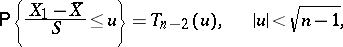
Since the statistic | Since the statistic | ||
| − | + | <table class="eq" style="width:100%;"> <tr><td valign="top" style="width:94%;text-align:center;"><img align="absmiddle" border="0" src="https://www.encyclopediaofmath.org/legacyimages/r/r077/r077550/r07755052.png" /></td> </tr></table> | |
| − | |||
| − | |||
| − | |||
| − | |||
| − | |||
| − | |||
| − | |||
| − | |||
| − | |||
| − | |||
| − | |||
| − | |||
| − | |||
| − | |||
| − | |||
| − | |||
| − | |||
| − | |||
| − | + | which is complementary to <img align="absmiddle" border="0" src="https://www.encyclopediaofmath.org/legacyimages/r/r077/r077550/r07755053.png" />, has a uniform distribution on the <img align="absmiddle" border="0" src="https://www.encyclopediaofmath.org/legacyimages/r/r077/r077550/r07755054.png" />-dimensional sphere of radius <img align="absmiddle" border="0" src="https://www.encyclopediaofmath.org/legacyimages/r/r077/r077550/r07755055.png" /> and, therefore, depends neither on the unknown parameters <img align="absmiddle" border="0" src="https://www.encyclopediaofmath.org/legacyimages/r/r077/r077550/r07755056.png" /> and <img align="absmiddle" border="0" src="https://www.encyclopediaofmath.org/legacyimages/r/r077/r077550/r07755057.png" /> nor on <img align="absmiddle" border="0" src="https://www.encyclopediaofmath.org/legacyimages/r/r077/r077550/r07755058.png" />, the same is true for <img align="absmiddle" border="0" src="https://www.encyclopediaofmath.org/legacyimages/r/r077/r077550/r07755059.png" /> and | |
| − | |||
| − | + | <table class="eq" style="width:100%;"> <tr><td valign="top" style="width:94%;text-align:center;"><img align="absmiddle" border="0" src="https://www.encyclopediaofmath.org/legacyimages/r/r077/r077550/r07755060.png" /></td> <td valign="top" style="width:5%;text-align:right;">(2)</td></tr></table> | |
| − | |||
| − | |||
| − | |||
| − | |||
where | where | ||
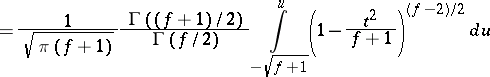
| − | + | <table class="eq" style="width:100%;"> <tr><td valign="top" style="width:94%;text-align:center;"><img align="absmiddle" border="0" src="https://www.encyclopediaofmath.org/legacyimages/r/r077/r077550/r07755061.png" /></td> <td valign="top" style="width:5%;text-align:right;">(3)</td></tr></table> | |
| − | |||
| − | |||
| − | + | <table class="eq" style="width:100%;"> <tr><td valign="top" style="width:94%;text-align:center;"><img align="absmiddle" border="0" src="https://www.encyclopediaofmath.org/legacyimages/r/r077/r077550/r07755062.png" /></td> </tr></table> | |
| − | = | ||
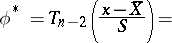
| − | + | is the Thompson distribution with <img align="absmiddle" border="0" src="https://www.encyclopediaofmath.org/legacyimages/r/r077/r077550/r07755063.png" /> degrees of freedom. Thus, (1)–(3) imply that the best unbiased estimator for <img align="absmiddle" border="0" src="https://www.encyclopediaofmath.org/legacyimages/r/r077/r077550/r07755064.png" /> obtained from <img align="absmiddle" border="0" src="https://www.encyclopediaofmath.org/legacyimages/r/r077/r077550/r07755065.png" /> independent observations <img align="absmiddle" border="0" src="https://www.encyclopediaofmath.org/legacyimages/r/r077/r077550/r07755066.png" /> is | |
| − | |||
| − | |||
| − | |||
| − | |||
| − | |||
| − | |||
| − | |||
| − | + | <table class="eq" style="width:100%;"> <tr><td valign="top" style="width:94%;text-align:center;"><img align="absmiddle" border="0" src="https://www.encyclopediaofmath.org/legacyimages/r/r077/r077550/r07755067.png" /></td> </tr></table> | |
| − | |||
| − | |||
| − | |||
| − | |||
| − | + | <table class="eq" style="width:100%;"> <tr><td valign="top" style="width:94%;text-align:center;"><img align="absmiddle" border="0" src="https://www.encyclopediaofmath.org/legacyimages/r/r077/r077550/r07755068.png" /></td> </tr></table> | |
| − | |||
| − | |||
| − | |||
| − | + | where <img align="absmiddle" border="0" src="https://www.encyclopediaofmath.org/legacyimages/r/r077/r077550/r07755069.png" /> is the Student distribution with <img align="absmiddle" border="0" src="https://www.encyclopediaofmath.org/legacyimages/r/r077/r077550/r07755070.png" /> degrees of freedom. | |
| − | + | ====References==== | |
| − | + | <table><TR><TD valign="top">[1]</TD> <TD valign="top"> A.N. Kolmogorov, "Unbiased estimates" ''Izv. Akad. Nauk SSSR Ser. Mat.'' , '''14''' : 4 (1950) pp. 303–326 (In Russian)</TD></TR><TR><TD valign="top">[2]</TD> <TD valign="top"> C.R. Rao, "Linear statistical inference and its applications" , Wiley (1965)</TD></TR><TR><TD valign="top">[3]</TD> <TD valign="top"> B.L. van der Waerden, "Mathematische Statistik" , Springer (1957)</TD></TR><TR><TD valign="top">[4]</TD> <TD valign="top"> D. Blackwell, "Conditional expectation and unbiased sequential estimation" ''Ann. Math. Stat.'' , '''18''' (1947) pp. 105–110</TD></TR></table> | |
| − | |||
| − | |||
| − | = | ||
| − | |||
| − | |||
| − | |||
| − | |||
| − | |||
| − | |||
| − | |||
| − | |||
| − | |||
| − | |||
| − | |||
====Comments==== | ====Comments==== | ||
In the Western literature this theorem is mostly referred to as the Rao–Blackwell theorem. | In the Western literature this theorem is mostly referred to as the Rao–Blackwell theorem. | ||
Revision as of 14:53, 7 June 2020
A proposition from the theory of statistical estimation on which a method for the improvement of unbiased statistical estimators is based.
Let  be a random variable with values in a sample space
  ,
,  , such that the family of probability distributions
 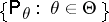 has a sufficient statistic
  , and let
  be a vector statistic with finite matrix of second moments. Then the mean
  of
of  exists and, moreover, the conditional mean
 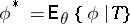 is an unbiased estimator for
  , that is,
 |
The Rao–Blackwell–Kolmogorov theorem states that under these conditions the quadratic risk of  does not exceed the quadratic risk of
  , uniformly in
  , i.e. for any vector
  of the same dimension as
  , the inequality
 |
 |
holds for any  . In particular, if
  is a one-dimensional statistic, then for any
  the variance
  of
of  does not exceed the variance
  of
of  .
.
In the most general situation the Rao–Blackwell–Kolmogorov theorem states that averaging over a sufficient statistic does not lead to an increase of the risk with respect to any convex loss function. This implies that good statistical estimators should be looked for only in terms of sufficient statistics, that is, in the class of functions of sufficient statistics.
In case the family  is complete, that is, when the function of
  that is almost-everywhere equal to zero is the only unbiased estimator based on
  for zero, the unbiased estimator with uniformly minimal risk provided by the Rao–Blackwell–Kolmogorov theorem is unique. Thus, the Rao–Blackwell–Kolmogorov theorem gives a recipe for constructing best unbiased estimators: one has to take some unbiased estimator and then average it over a sufficient statistic. That is how the best unbiased estimator for the distribution function of the normal law is constructed in the following example, which is due to A.N. Kolmogorov.
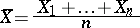
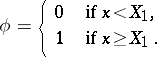
Example. Given a realization of a random vector  whose components
  ,
,  ,
,  , are independent random variables subject to the same normal law
  , it is required to estimate the distribution function
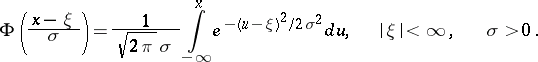 |
The parameters  and
and  are supposed to be unknown. Since the family
 |
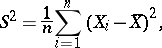
of normal laws has a complete sufficient statistic  , where
 |
and
 |
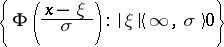
the Rao–Blackwell–Kolmogorov theorem can be used for the construction of the best unbiased estimator for the distribution function 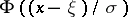 . As an initial statistic
  one may use, e.g., the empirical distribution function constructed from an arbitrary component
  of
of  :
:
 |
This is a trivial unbiased estimator for  , since
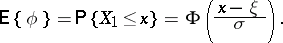 |
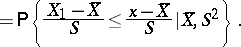
Averaging of  over the sufficient statistic
  gives the estimator
 | (1) |
 |
Since the statistic
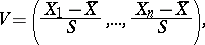 |
which is complementary to  , has a uniform distribution on the
  -dimensional sphere of radius
  and, therefore, depends neither on the unknown parameters
  and
and  nor on
  , the same is true for
  and
and
 | (2) |
where
 | (3) |
 |
is the Thompson distribution with  degrees of freedom. Thus, (1)–(3) imply that the best unbiased estimator for
  obtained from
  independent observations
  is
is
 |
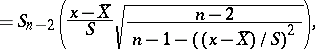 |
where  is the Student distribution with
  degrees of freedom.
References
| [1] | A.N. Kolmogorov, "Unbiased estimates" Izv. Akad. Nauk SSSR Ser. Mat. , 14 : 4 (1950) pp. 303–326 (In Russian) |
| [2] | C.R. Rao, "Linear statistical inference and its applications" , Wiley (1965) |
| [3] | B.L. van der Waerden, "Mathematische Statistik" , Springer (1957) |
| [4] | D. Blackwell, "Conditional expectation and unbiased sequential estimation" Ann. Math. Stat. , 18 (1947) pp. 105–110 |
Comments
In the Western literature this theorem is mostly referred to as the Rao–Blackwell theorem.
Rao-Blackwell-Kolmogorov theorem. Encyclopedia of Mathematics. URL: http://encyclopediaofmath.org/index.php?title=Rao-Blackwell-Kolmogorov_theorem&oldid=49389