Difference between revisions of "Pontryagin maximum principle"
(Importing text file) |
(some TeX) |
||
| Line 1: | Line 1: | ||
| − | + | {{TEX|part}} | |
| − | + | Relations describing necessary conditions for a strong maximum in a non-classical [[variational problem]] in the [[Optimal control, mathematical theory of|mathematical theory of optimal control]]. It was first formulated in 1956 by L.S. Pontryagin <ref name="Pontryagin" />. | |
| − | + | The proposed formulation of the Pontryagin maximum principle corresponds to the following problem of optimal control. Given a system of [[ordinary differential equation]]s | |
| − | + | \begin{equation}\label{eq:1} | |
| − | where <img align="absmiddle" border="0" src="https://www.encyclopediaofmath.org/legacyimages/p/p073/p073780/p0737802.png" /> is a phase vector, <img align="absmiddle" border="0" src="https://www.encyclopediaofmath.org/legacyimages/p/p073/p073780/p0737803.png" /> is a control parameter and <img align="absmiddle" border="0" src="https://www.encyclopediaofmath.org/legacyimages/p/p073/p073780/p0737804.png" /> is a continuous vector function in the variables <img align="absmiddle" border="0" src="https://www.encyclopediaofmath.org/legacyimages/p/p073/p073780/p0737805.png" /> that is continuously differentiable with respect to <img align="absmiddle" border="0" src="https://www.encyclopediaofmath.org/legacyimages/p/p073/p073780/p0737806.png" />. A certain set <img align="absmiddle" border="0" src="https://www.encyclopediaofmath.org/legacyimages/p/p073/p073780/p0737807.png" /> of admissible values of the control parameter <img align="absmiddle" border="0" src="https://www.encyclopediaofmath.org/legacyimages/p/p073/p073780/p0737808.png" /> in the space <img align="absmiddle" border="0" src="https://www.encyclopediaofmath.org/legacyimages/p/p073/p073780/p0737809.png" /> is given; two points <img align="absmiddle" border="0" src="https://www.encyclopediaofmath.org/legacyimages/p/p073/p073780/p07378010.png" /> and <img align="absmiddle" border="0" src="https://www.encyclopediaofmath.org/legacyimages/p/p073/p073780/p07378011.png" /> in the phase space <img align="absmiddle" border="0" src="https://www.encyclopediaofmath.org/legacyimages/p/p073/p073780/p07378012.png" /> are given; the initial time <img align="absmiddle" border="0" src="https://www.encyclopediaofmath.org/legacyimages/p/p073/p073780/p07378013.png" /> is fixed. Any piecewise-continuous function <img align="absmiddle" border="0" src="https://www.encyclopediaofmath.org/legacyimages/p/p073/p073780/p07378014.png" />, <img align="absmiddle" border="0" src="https://www.encyclopediaofmath.org/legacyimages/p/p073/p073780/p07378015.png" />, with values in <img align="absmiddle" border="0" src="https://www.encyclopediaofmath.org/legacyimages/p/p073/p073780/p07378016.png" />, is called an admissible control. One says that an admissible control <img align="absmiddle" border="0" src="https://www.encyclopediaofmath.org/legacyimages/p/p073/p073780/p07378017.png" /> transfers the phase point from the position <img align="absmiddle" border="0" src="https://www.encyclopediaofmath.org/legacyimages/p/p073/p073780/p07378018.png" /> to the position <img align="absmiddle" border="0" src="https://www.encyclopediaofmath.org/legacyimages/p/p073/p073780/p07378019.png" /> (<img align="absmiddle" border="0" src="https://www.encyclopediaofmath.org/legacyimages/p/p073/p073780/p07378020.png" />) if the corresponding solution <img align="absmiddle" border="0" src="https://www.encyclopediaofmath.org/legacyimages/p/p073/p073780/p07378021.png" /> of the system | + | \dot{x}=f(x,u), |
| + | \end{equation} | ||
| + | where <img align="absmiddle" border="0" src="https://www.encyclopediaofmath.org/legacyimages/p/p073/p073780/p0737802.png" /> is a phase vector, <img align="absmiddle" border="0" src="https://www.encyclopediaofmath.org/legacyimages/p/p073/p073780/p0737803.png" /> is a control parameter and <img align="absmiddle" border="0" src="https://www.encyclopediaofmath.org/legacyimages/p/p073/p073780/p0737804.png" /> is a continuous vector function in the variables <img align="absmiddle" border="0" src="https://www.encyclopediaofmath.org/legacyimages/p/p073/p073780/p0737805.png" /> that is continuously differentiable with respect to <img align="absmiddle" border="0" src="https://www.encyclopediaofmath.org/legacyimages/p/p073/p073780/p0737806.png" />. A certain set <img align="absmiddle" border="0" src="https://www.encyclopediaofmath.org/legacyimages/p/p073/p073780/p0737807.png" /> of admissible values of the control parameter <img align="absmiddle" border="0" src="https://www.encyclopediaofmath.org/legacyimages/p/p073/p073780/p0737808.png" /> in the space <img align="absmiddle" border="0" src="https://www.encyclopediaofmath.org/legacyimages/p/p073/p073780/p0737809.png" /> is given; two points <img align="absmiddle" border="0" src="https://www.encyclopediaofmath.org/legacyimages/p/p073/p073780/p07378010.png" /> and <img align="absmiddle" border="0" src="https://www.encyclopediaofmath.org/legacyimages/p/p073/p073780/p07378011.png" /> in the phase space <img align="absmiddle" border="0" src="https://www.encyclopediaofmath.org/legacyimages/p/p073/p073780/p07378012.png" /> are given; the initial time <img align="absmiddle" border="0" src="https://www.encyclopediaofmath.org/legacyimages/p/p073/p073780/p07378013.png" /> is fixed. Any piecewise-continuous function <img align="absmiddle" border="0" src="https://www.encyclopediaofmath.org/legacyimages/p/p073/p073780/p07378014.png" />, <img align="absmiddle" border="0" src="https://www.encyclopediaofmath.org/legacyimages/p/p073/p073780/p07378015.png" />, with values in <img align="absmiddle" border="0" src="https://www.encyclopediaofmath.org/legacyimages/p/p073/p073780/p07378016.png" />, is called an admissible control. One says that an admissible control <img align="absmiddle" border="0" src="https://www.encyclopediaofmath.org/legacyimages/p/p073/p073780/p07378017.png" /> transfers the phase point from the position <img align="absmiddle" border="0" src="https://www.encyclopediaofmath.org/legacyimages/p/p073/p073780/p07378018.png" /> to the position <img align="absmiddle" border="0" src="https://www.encyclopediaofmath.org/legacyimages/p/p073/p073780/p07378019.png" /> (<img align="absmiddle" border="0" src="https://www.encyclopediaofmath.org/legacyimages/p/p073/p073780/p07378020.png" />) if the corresponding solution <img align="absmiddle" border="0" src="https://www.encyclopediaofmath.org/legacyimages/p/p073/p073780/p07378021.png" /> of the system \eqref{eq:1} satisfying the initial condition <img align="absmiddle" border="0" src="https://www.encyclopediaofmath.org/legacyimages/p/p073/p073780/p07378022.png" /> is defined for all <img align="absmiddle" border="0" src="https://www.encyclopediaofmath.org/legacyimages/p/p073/p073780/p07378023.png" /> and if <img align="absmiddle" border="0" src="https://www.encyclopediaofmath.org/legacyimages/p/p073/p073780/p07378024.png" />. Among all admissible controls transferring the phase point from the position <img align="absmiddle" border="0" src="https://www.encyclopediaofmath.org/legacyimages/p/p073/p073780/p07378025.png" /> to the position <img align="absmiddle" border="0" src="https://www.encyclopediaofmath.org/legacyimages/p/p073/p073780/p07378026.png" /> it is required to find an optimal control, i.e. a function <img align="absmiddle" border="0" src="https://www.encyclopediaofmath.org/legacyimages/p/p073/p073780/p07378027.png" /> for which the functional | ||
<table class="eq" style="width:100%;"> <tr><td valign="top" style="width:94%;text-align:center;"><img align="absmiddle" border="0" src="https://www.encyclopediaofmath.org/legacyimages/p/p073/p073780/p07378028.png" /></td> <td valign="top" style="width:5%;text-align:right;">(2)</td></tr></table> | <table class="eq" style="width:100%;"> <tr><td valign="top" style="width:94%;text-align:center;"><img align="absmiddle" border="0" src="https://www.encyclopediaofmath.org/legacyimages/p/p073/p073780/p07378028.png" /></td> <td valign="top" style="width:5%;text-align:right;">(2)</td></tr></table> | ||
| − | takes least possible value. Here <img align="absmiddle" border="0" src="https://www.encyclopediaofmath.org/legacyimages/p/p073/p073780/p07378029.png" /> is a given function from the same class as <img align="absmiddle" border="0" src="https://www.encyclopediaofmath.org/legacyimages/p/p073/p073780/p07378030.png" />, <img align="absmiddle" border="0" src="https://www.encyclopediaofmath.org/legacyimages/p/p073/p073780/p07378031.png" /> is the solution of the system | + | takes least possible value. Here <img align="absmiddle" border="0" src="https://www.encyclopediaofmath.org/legacyimages/p/p073/p073780/p07378029.png" /> is a given function from the same class as <img align="absmiddle" border="0" src="https://www.encyclopediaofmath.org/legacyimages/p/p073/p073780/p07378030.png" />, <img align="absmiddle" border="0" src="https://www.encyclopediaofmath.org/legacyimages/p/p073/p073780/p07378031.png" /> is the solution of the system \eqref{eq:1} with the initial condition <img align="absmiddle" border="0" src="https://www.encyclopediaofmath.org/legacyimages/p/p073/p073780/p07378032.png" /> corresponding to the control <img align="absmiddle" border="0" src="https://www.encyclopediaofmath.org/legacyimages/p/p073/p073780/p07378033.png" />, and <img align="absmiddle" border="0" src="https://www.encyclopediaofmath.org/legacyimages/p/p073/p073780/p07378034.png" /> is the time at which this solution passes through <img align="absmiddle" border="0" src="https://www.encyclopediaofmath.org/legacyimages/p/p073/p073780/p07378035.png" />. The problem consists of finding a pair consisting of the optimal control <img align="absmiddle" border="0" src="https://www.encyclopediaofmath.org/legacyimages/p/p073/p073780/p07378036.png" /> and the corresponding optimal trajectory <img align="absmiddle" border="0" src="https://www.encyclopediaofmath.org/legacyimages/p/p073/p073780/p07378037.png" /> of \eqref{eq:1}. |
Let | Let | ||
| Line 19: | Line 21: | ||
<table class="eq" style="width:100%;"> <tr><td valign="top" style="width:94%;text-align:center;"><img align="absmiddle" border="0" src="https://www.encyclopediaofmath.org/legacyimages/p/p073/p073780/p07378046.png" /></td> <td valign="top" style="width:5%;text-align:right;">(3)</td></tr></table> | <table class="eq" style="width:100%;"> <tr><td valign="top" style="width:94%;text-align:center;"><img align="absmiddle" border="0" src="https://www.encyclopediaofmath.org/legacyimages/p/p073/p073780/p07378046.png" /></td> <td valign="top" style="width:5%;text-align:right;">(3)</td></tr></table> | ||
| − | (the first equation in (3) is the system | + | (the first equation in (3) is the system \eqref{eq:1}). Let |
<table class="eq" style="width:100%;"> <tr><td valign="top" style="width:94%;text-align:center;"><img align="absmiddle" border="0" src="https://www.encyclopediaofmath.org/legacyimages/p/p073/p073780/p07378047.png" /></td> </tr></table> | <table class="eq" style="width:100%;"> <tr><td valign="top" style="width:94%;text-align:center;"><img align="absmiddle" border="0" src="https://www.encyclopediaofmath.org/legacyimages/p/p073/p073780/p07378047.png" /></td> </tr></table> | ||
| − | The Pontryagin maximum principle states: If <img align="absmiddle" border="0" src="https://www.encyclopediaofmath.org/legacyimages/p/p073/p073780/p07378048.png" /> (<img align="absmiddle" border="0" src="https://www.encyclopediaofmath.org/legacyimages/p/p073/p073780/p07378049.png" />) is a solution of the optimal control problem | + | The Pontryagin maximum principle states: If <img align="absmiddle" border="0" src="https://www.encyclopediaofmath.org/legacyimages/p/p073/p073780/p07378048.png" /> (<img align="absmiddle" border="0" src="https://www.encyclopediaofmath.org/legacyimages/p/p073/p073780/p07378049.png" />) is a solution of the optimal control problem \eqref{eq:1}, (2) (<img align="absmiddle" border="0" src="https://www.encyclopediaofmath.org/legacyimages/p/p073/p073780/p07378050.png" />, <img align="absmiddle" border="0" src="https://www.encyclopediaofmath.org/legacyimages/p/p073/p073780/p07378051.png" />), then there exists a non-zero absolutely-continuous function <img align="absmiddle" border="0" src="https://www.encyclopediaofmath.org/legacyimages/p/p073/p073780/p07378052.png" /> such that <img align="absmiddle" border="0" src="https://www.encyclopediaofmath.org/legacyimages/p/p073/p073780/p07378053.png" /> satisfy system (3) in <img align="absmiddle" border="0" src="https://www.encyclopediaofmath.org/legacyimages/p/p073/p073780/p07378054.png" />, such that for almost-all <img align="absmiddle" border="0" src="https://www.encyclopediaofmath.org/legacyimages/p/p073/p073780/p07378055.png" /> the function <img align="absmiddle" border="0" src="https://www.encyclopediaofmath.org/legacyimages/p/p073/p073780/p07378056.png" /> attains its maximum: |
<table class="eq" style="width:100%;"> <tr><td valign="top" style="width:94%;text-align:center;"><img align="absmiddle" border="0" src="https://www.encyclopediaofmath.org/legacyimages/p/p073/p073780/p07378057.png" /></td> <td valign="top" style="width:5%;text-align:right;">(4)</td></tr></table> | <table class="eq" style="width:100%;"> <tr><td valign="top" style="width:94%;text-align:center;"><img align="absmiddle" border="0" src="https://www.encyclopediaofmath.org/legacyimages/p/p073/p073780/p07378057.png" /></td> <td valign="top" style="width:5%;text-align:right;">(4)</td></tr></table> | ||
| Line 39: | Line 41: | ||
hold. | hold. | ||
| − | From the above statement follows the maximum principle for the time-optimal problem (<img align="absmiddle" border="0" src="https://www.encyclopediaofmath.org/legacyimages/p/p073/p073780/p07378063.png" />, <img align="absmiddle" border="0" src="https://www.encyclopediaofmath.org/legacyimages/p/p073/p073780/p07378064.png" />). This statement admits a natural generalization to non-autonomous systems, problems with variable end-points and problems with restricted phase coordinates (<img align="absmiddle" border="0" src="https://www.encyclopediaofmath.org/legacyimages/p/p073/p073780/p07378065.png" />, where <img align="absmiddle" border="0" src="https://www.encyclopediaofmath.org/legacyimages/p/p073/p073780/p07378066.png" /> is a closed set in the phase space <img align="absmiddle" border="0" src="https://www.encyclopediaofmath.org/legacyimages/p/p073/p073780/p07378067.png" /> satisfying some additional restrictions | + | From the above statement follows the maximum principle for the time-optimal problem (<img align="absmiddle" border="0" src="https://www.encyclopediaofmath.org/legacyimages/p/p073/p073780/p07378063.png" />, <img align="absmiddle" border="0" src="https://www.encyclopediaofmath.org/legacyimages/p/p073/p073780/p07378064.png" />). This statement admits a natural generalization to non-autonomous systems, problems with variable end-points and problems with restricted phase coordinates (<img align="absmiddle" border="0" src="https://www.encyclopediaofmath.org/legacyimages/p/p073/p073780/p07378065.png" />, where <img align="absmiddle" border="0" src="https://www.encyclopediaofmath.org/legacyimages/p/p073/p073780/p07378066.png" /> is a closed set in the phase space <img align="absmiddle" border="0" src="https://www.encyclopediaofmath.org/legacyimages/p/p073/p073780/p07378067.png" /> satisfying some additional restrictions <ref name="Pontryagin" />. |
| − | Admitting closed sets <img align="absmiddle" border="0" src="https://www.encyclopediaofmath.org/legacyimages/p/p073/p073780/p07378068.png" /> (in particular, these regions can be determined by systems of non-strict inequalities) makes the problem under consideration non-classical. The fundamental necessary conditions from the classical calculus of variations with ordinary derivative follow from the Pontryagin maximum principle (see | + | Admitting closed sets <img align="absmiddle" border="0" src="https://www.encyclopediaofmath.org/legacyimages/p/p073/p073780/p07378068.png" /> (in particular, these regions can be determined by systems of non-strict inequalities) makes the problem under consideration non-classical. The fundamental necessary conditions from the classical calculus of variations with ordinary derivative follow from the Pontryagin maximum principle (see <ref name="Pontryagin" /> and also [[Weierstrass conditions (for a variational extremum)|Weierstrass conditions (for a variational extremum)]]). |
| − | A widely used proof of the above formulation of the Pontryagin maximum principle, based on needle variations (i.e. one considers admissible controls arbitrarily deviating from the optimal one but only on a finite number of small time intervals), consists of linearization of the problem in a neighbourhood of the optimal solution, construction of a convex cone of variations of the optimal trajectory, and subsequent application of the theorem on separated convex cones | + | A widely used proof of the above formulation of the Pontryagin maximum principle, based on needle variations (i.e. one considers admissible controls arbitrarily deviating from the optimal one but only on a finite number of small time intervals), consists of linearization of the problem in a neighbourhood of the optimal solution, construction of a convex cone of variations of the optimal trajectory, and subsequent application of the theorem on separated convex cones <ref name="Pontryagin" />. The corresponding condition is then rewritten in the analytical form (3), (4) in terms of the maximum of the Hamiltonian <img align="absmiddle" border="0" src="https://www.encyclopediaofmath.org/legacyimages/p/p073/p073780/p07378069.png" /> of the phase variables <img align="absmiddle" border="0" src="https://www.encyclopediaofmath.org/legacyimages/p/p073/p073780/p07378070.png" />, the controls <img align="absmiddle" border="0" src="https://www.encyclopediaofmath.org/legacyimages/p/p073/p073780/p07378071.png" /> and the adjoint variables <img align="absmiddle" border="0" src="https://www.encyclopediaofmath.org/legacyimages/p/p073/p073780/p07378072.png" />, which play the same role as the [[Lagrange multipliers|Lagrange multipliers]] in the classical calculus of variations. Effective application of the Pontryagin maximum principle often necessitates the solution of a two-point boundary value problem for (3). |
The most complete solution of the problem of optimal control was obtained in the case of certain linear systems, for which the relations in the Pontryagin maximum principle are not only necessary but also sufficient optimality conditions. | The most complete solution of the problem of optimal control was obtained in the case of certain linear systems, for which the relations in the Pontryagin maximum principle are not only necessary but also sufficient optimality conditions. | ||
| Line 49: | Line 51: | ||
There are numerous generalizations of the Pontryagin maximum principle; for instance, in the direction of more complicated non-classical constraints (including mixed constraints imposed on the controls and phase coordinates, functional and different integral constraints), in studies of the sufficiency of the corresponding constraints, in the consideration of generalized solutions, so-called sliding regimes, systems of differential equations with non-smooth right-hand side, differential inclusions, optimal control problems for discrete systems and systems with an infinite number of degrees of freedom, in particular, described by partial differential equations, equations with an after effect (including equations with a delay), evolution equations in a Banach space, etc. The latter lead to new classes of variations of the corresponding functionals, the introduction of the so-called integral maximum principle, the linearized maximum principle, etc. Rather general classes of variational problems with non-classical constraints (including non-strict inequalities) or with non-smooth functionals are usually called problems of Pontryagin type. The discovery of the Pontryagin maximum principle initiated the development of mathematical optimal control theory. It stimulated new research in the field of differential equations, functional analysis and extremal problems, computational mathematics and other related domains. | There are numerous generalizations of the Pontryagin maximum principle; for instance, in the direction of more complicated non-classical constraints (including mixed constraints imposed on the controls and phase coordinates, functional and different integral constraints), in studies of the sufficiency of the corresponding constraints, in the consideration of generalized solutions, so-called sliding regimes, systems of differential equations with non-smooth right-hand side, differential inclusions, optimal control problems for discrete systems and systems with an infinite number of degrees of freedom, in particular, described by partial differential equations, equations with an after effect (including equations with a delay), evolution equations in a Banach space, etc. The latter lead to new classes of variations of the corresponding functionals, the introduction of the so-called integral maximum principle, the linearized maximum principle, etc. Rather general classes of variational problems with non-classical constraints (including non-strict inequalities) or with non-smooth functionals are usually called problems of Pontryagin type. The discovery of the Pontryagin maximum principle initiated the development of mathematical optimal control theory. It stimulated new research in the field of differential equations, functional analysis and extremal problems, computational mathematics and other related domains. | ||
| − | |||
| − | |||
| + | |||
| + | ====Comments==== | ||
| + | |||
| + | In the Western literature the Pontryagin maximum principle is also simply known as the minimum principle. (Cf. [[Optimal control, mathematical theory of]]) | ||
| − | |||
| − | |||
====References==== | ====References==== | ||
| − | <table><TR><TD valign="top">[a1]</TD> <TD valign="top"> W.H. Fleming, R.W. Rishel, "Deterministic and stochastic optimal control" , Springer (1975)</TD></TR><TR><TD valign="top">[a2]</TD> <TD valign="top"> L. Markus, "Foundations of optimal control theory" , Wiley (1967)</TD></TR><TR><TD valign="top">[a3]</TD> <TD valign="top"> L.D. Berkovitz, "Optimal control theory" , Springer (1974)</TD></TR><TR><TD valign="top">[a4]</TD> <TD valign="top"> L. Cesari, "Optimization - Theory and applications" , Springer (1983)</TD></TR><TR><TD valign="top">[a5]</TD> <TD valign="top"> F. Clarke, "Optimization and nonsmooth analysis" , Wiley (1983)</TD></TR></table> | + | |
| + | <references> | ||
| + | <ref name="Pontryagin">L.S. Pontryagin, V.G. Boltayanskii, R.V. Gamkrelidze, E.F. Mishchenko, "The mathematical theory of optimal processes" , Wiley (1962) (Translated from Russian)</ref> | ||
| + | </references> | ||
| + | |||
| + | <table> | ||
| + | <TR><TD valign="top">[a1]</TD> <TD valign="top"> W.H. Fleming, R.W. Rishel, "Deterministic and stochastic optimal control" , Springer (1975)</TD></TR> | ||
| + | <TR><TD valign="top">[a2]</TD> <TD valign="top"> L. Markus, "Foundations of optimal control theory" , Wiley (1967)</TD></TR> | ||
| + | <TR><TD valign="top">[a3]</TD> <TD valign="top"> L.D. Berkovitz, "Optimal control theory" , Springer (1974)</TD></TR> | ||
| + | <TR><TD valign="top">[a4]</TD> <TD valign="top"> L. Cesari, "Optimization - Theory and applications" , Springer (1983)</TD></TR> | ||
| + | <TR><TD valign="top">[a5]</TD> <TD valign="top"> F. Clarke, "Optimization and nonsmooth analysis" , Wiley (1983)</TD></TR> | ||
| + | </table> | ||
Revision as of 11:55, 7 June 2016
Relations describing necessary conditions for a strong maximum in a non-classical variational problem in the mathematical theory of optimal control. It was first formulated in 1956 by L.S. Pontryagin [1].
The proposed formulation of the Pontryagin maximum principle corresponds to the following problem of optimal control. Given a system of ordinary differential equations
\begin{equation}\label{eq:1}
\dot{x}=f(x,u),
\end{equation}
where  is a phase vector,
  is a control parameter and
  is a continuous vector function in the variables
  that is continuously differentiable with respect to
  . A certain set
  of admissible values of the control parameter
  in the space
  is given; two points
  and
and  in the phase space
  are given; the initial time
  is fixed. Any piecewise-continuous function
  ,
,  , with values in
  , is called an admissible control. One says that an admissible control
  transfers the phase point from the position
  to the position
  (
( ) if the corresponding solution
  of the system \eqref{eq:1} satisfying the initial condition
  is defined for all
  and if
  . Among all admissible controls transferring the phase point from the position
  to the position
  it is required to find an optimal control, i.e. a function
  for which the functional
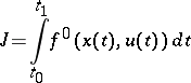 | (2) |
takes least possible value. Here  is a given function from the same class as
  ,
,  is the solution of the system \eqref{eq:1} with the initial condition
  corresponding to the control
  , and
, and  is the time at which this solution passes through
  . The problem consists of finding a pair consisting of the optimal control
  and the corresponding optimal trajectory
  of \eqref{eq:1}.
Let
 |
be a scalar function (Hamiltonian) of the variables  , where
 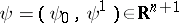 ,
,  ,
,  ,
,  . To the function
  corresponds a canonical (Hamiltonian) system (with respect to
  )
)
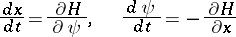 | (3) |
(the first equation in (3) is the system \eqref{eq:1}). Let
 |
The Pontryagin maximum principle states: If  (
( ) is a solution of the optimal control problem \eqref{eq:1}, (2) (
 ,
,  ), then there exists a non-zero absolutely-continuous function
  such that
 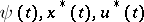 satisfy system (3) in
  , such that for almost-all
  the function
  attains its maximum:
 | (4) |
and such that at the terminal time  the conditions
 | (5) |
are satisfied.
If the functions  satisfy the relations (3), (4) (i.e.
  are Pontryagin extremal), then the conditions
 |
hold.
From the above statement follows the maximum principle for the time-optimal problem ( ,
,  ). This statement admits a natural generalization to non-autonomous systems, problems with variable end-points and problems with restricted phase coordinates (
 , where
  is a closed set in the phase space
  satisfying some additional restrictions [1].
Admitting closed sets  (in particular, these regions can be determined by systems of non-strict inequalities) makes the problem under consideration non-classical. The fundamental necessary conditions from the classical calculus of variations with ordinary derivative follow from the Pontryagin maximum principle (see [1] and also Weierstrass conditions (for a variational extremum)).
A widely used proof of the above formulation of the Pontryagin maximum principle, based on needle variations (i.e. one considers admissible controls arbitrarily deviating from the optimal one but only on a finite number of small time intervals), consists of linearization of the problem in a neighbourhood of the optimal solution, construction of a convex cone of variations of the optimal trajectory, and subsequent application of the theorem on separated convex cones [1]. The corresponding condition is then rewritten in the analytical form (3), (4) in terms of the maximum of the Hamiltonian  of the phase variables
  , the controls
  and the adjoint variables
  , which play the same role as the Lagrange multipliers in the classical calculus of variations. Effective application of the Pontryagin maximum principle often necessitates the solution of a two-point boundary value problem for (3).
The most complete solution of the problem of optimal control was obtained in the case of certain linear systems, for which the relations in the Pontryagin maximum principle are not only necessary but also sufficient optimality conditions.
There are numerous generalizations of the Pontryagin maximum principle; for instance, in the direction of more complicated non-classical constraints (including mixed constraints imposed on the controls and phase coordinates, functional and different integral constraints), in studies of the sufficiency of the corresponding constraints, in the consideration of generalized solutions, so-called sliding regimes, systems of differential equations with non-smooth right-hand side, differential inclusions, optimal control problems for discrete systems and systems with an infinite number of degrees of freedom, in particular, described by partial differential equations, equations with an after effect (including equations with a delay), evolution equations in a Banach space, etc. The latter lead to new classes of variations of the corresponding functionals, the introduction of the so-called integral maximum principle, the linearized maximum principle, etc. Rather general classes of variational problems with non-classical constraints (including non-strict inequalities) or with non-smooth functionals are usually called problems of Pontryagin type. The discovery of the Pontryagin maximum principle initiated the development of mathematical optimal control theory. It stimulated new research in the field of differential equations, functional analysis and extremal problems, computational mathematics and other related domains.
Comments
In the Western literature the Pontryagin maximum principle is also simply known as the minimum principle. (Cf. Optimal control, mathematical theory of)
References
| [a1] | W.H. Fleming, R.W. Rishel, "Deterministic and stochastic optimal control" , Springer (1975) |
| [a2] | L. Markus, "Foundations of optimal control theory" , Wiley (1967) |
| [a3] | L.D. Berkovitz, "Optimal control theory" , Springer (1974) |
| [a4] | L. Cesari, "Optimization - Theory and applications" , Springer (1983) |
| [a5] | F. Clarke, "Optimization and nonsmooth analysis" , Wiley (1983) |
Pontryagin maximum principle. Encyclopedia of Mathematics. URL: http://encyclopediaofmath.org/index.php?title=Pontryagin_maximum_principle&oldid=38941