Difference between revisions of "Parametrix method"
Ulf Rehmann (talk | contribs) m (tex encoded by computer) |
Ulf Rehmann (talk | contribs) m (Undo revision 48129 by Ulf Rehmann (talk)) Tag: Undo |
||
| Line 1: | Line 1: | ||
| − | |||
| − | |||
| − | |||
| − | |||
| − | |||
| − | |||
| − | |||
| − | |||
| − | |||
| − | |||
| − | |||
| − | |||
One of the methods for studying boundary value problems for differential equations with variable coefficients by means of integral equations. | One of the methods for studying boundary value problems for differential equations with variable coefficients by means of integral equations. | ||
| − | Suppose that in some region | + | Suppose that in some region <img align="absmiddle" border="0" src="https://www.encyclopediaofmath.org/legacyimages/p/p071/p071570/p0715701.png" /> of the <img align="absmiddle" border="0" src="https://www.encyclopediaofmath.org/legacyimages/p/p071/p071570/p0715702.png" />-dimensional Euclidean space <img align="absmiddle" border="0" src="https://www.encyclopediaofmath.org/legacyimages/p/p071/p071570/p0715703.png" /> one considers an elliptic differential operator (cf. [[Elliptic partial differential equation|Elliptic partial differential equation]]) of order <img align="absmiddle" border="0" src="https://www.encyclopediaofmath.org/legacyimages/p/p071/p071570/p0715704.png" />, |
| − | of the | ||
| − | dimensional Euclidean space | ||
| − | one considers an elliptic differential operator (cf. [[Elliptic partial differential equation|Elliptic partial differential equation]]) of order | ||
| − | + | <table class="eq" style="width:100%;"> <tr><td valign="top" style="width:94%;text-align:center;"><img align="absmiddle" border="0" src="https://www.encyclopediaofmath.org/legacyimages/p/p071/p071570/p0715705.png" /></td> <td valign="top" style="width:5%;text-align:right;">(1)</td></tr></table> | |
| − | |||
| − | |||
| − | In (1) the symbol | + | In (1) the symbol <img align="absmiddle" border="0" src="https://www.encyclopediaofmath.org/legacyimages/p/p071/p071570/p0715706.png" /> is a multi-index, <img align="absmiddle" border="0" src="https://www.encyclopediaofmath.org/legacyimages/p/p071/p071570/p0715707.png" />, where the <img align="absmiddle" border="0" src="https://www.encyclopediaofmath.org/legacyimages/p/p071/p071570/p0715708.png" /> are non-negative integers, <img align="absmiddle" border="0" src="https://www.encyclopediaofmath.org/legacyimages/p/p071/p071570/p0715709.png" />, <img align="absmiddle" border="0" src="https://www.encyclopediaofmath.org/legacyimages/p/p071/p071570/p07157010.png" />, <img align="absmiddle" border="0" src="https://www.encyclopediaofmath.org/legacyimages/p/p071/p071570/p07157011.png" />. With every operator (1) there is associated the homogeneous elliptic operator |
| − | is a multi-index, | ||
| − | where the | ||
| − | are non-negative integers, | ||
| − | |||
| − | |||
| − | With every operator (1) there is associated the homogeneous elliptic operator | ||
| − | + | <table class="eq" style="width:100%;"> <tr><td valign="top" style="width:94%;text-align:center;"><img align="absmiddle" border="0" src="https://www.encyclopediaofmath.org/legacyimages/p/p071/p071570/p07157012.png" /></td> </tr></table> | |
| − | |||
| − | |||
| − | |||
| − | with constant coefficients, where | + | with constant coefficients, where <img align="absmiddle" border="0" src="https://www.encyclopediaofmath.org/legacyimages/p/p071/p071570/p07157013.png" /> is an arbitrary fixed point. Let <img align="absmiddle" border="0" src="https://www.encyclopediaofmath.org/legacyimages/p/p071/p071570/p07157014.png" /> denote a [[Fundamental solution|fundamental solution]] of <img align="absmiddle" border="0" src="https://www.encyclopediaofmath.org/legacyimages/p/p071/p071570/p07157015.png" /> depending parametrically on <img align="absmiddle" border="0" src="https://www.encyclopediaofmath.org/legacyimages/p/p071/p071570/p07157016.png" />. Then the function <img align="absmiddle" border="0" src="https://www.encyclopediaofmath.org/legacyimages/p/p071/p071570/p07157017.png" /> is called the parametrix of the operator (1) with a singularity at <img align="absmiddle" border="0" src="https://www.encyclopediaofmath.org/legacyimages/p/p071/p071570/p07157018.png" />. |
| − | is an arbitrary fixed point. Let | ||
| − | denote a [[Fundamental solution|fundamental solution]] of | ||
| − | depending parametrically on | ||
| − | Then the function | ||
| − | is called the parametrix of the operator (1) with a singularity at | ||
In particular, for the second-order elliptic operator | In particular, for the second-order elliptic operator | ||
| − | + | <table class="eq" style="width:100%;"> <tr><td valign="top" style="width:94%;text-align:center;"><img align="absmiddle" border="0" src="https://www.encyclopediaofmath.org/legacyimages/p/p071/p071570/p07157019.png" /></td> </tr></table> | |
| − | |||
| − | |||
| − | |||
| − | |||
| − | |||
| − | |||
| − | |||
| − | |||
| − | one can take as parametrix with singularity at | + | one can take as parametrix with singularity at <img align="absmiddle" border="0" src="https://www.encyclopediaofmath.org/legacyimages/p/p071/p071570/p07157020.png" /> the Levi function |
| − | the Levi function | ||
| − | + | <table class="eq" style="width:100%;"> <tr><td valign="top" style="width:94%;text-align:center;"><img align="absmiddle" border="0" src="https://www.encyclopediaofmath.org/legacyimages/p/p071/p071570/p07157021.png" /></td> <td valign="top" style="width:5%;text-align:right;">(2)</td></tr></table> | |
| − | |||
| − | In (2), | + | In (2), <img align="absmiddle" border="0" src="https://www.encyclopediaofmath.org/legacyimages/p/p071/p071570/p07157022.png" />, <img align="absmiddle" border="0" src="https://www.encyclopediaofmath.org/legacyimages/p/p071/p071570/p07157023.png" /> is the determinant of the matrix <img align="absmiddle" border="0" src="https://www.encyclopediaofmath.org/legacyimages/p/p071/p071570/p07157024.png" />, |
| − | |||
| − | is the determinant of the matrix | ||
| − | + | <table class="eq" style="width:100%;"> <tr><td valign="top" style="width:94%;text-align:center;"><img align="absmiddle" border="0" src="https://www.encyclopediaofmath.org/legacyimages/p/p071/p071570/p07157025.png" /></td> </tr></table> | |
| − | |||
| − | |||
| − | and | + | and <img align="absmiddle" border="0" src="https://www.encyclopediaofmath.org/legacyimages/p/p071/p071570/p07157026.png" /> are the elements of the matrix inverse to <img align="absmiddle" border="0" src="https://www.encyclopediaofmath.org/legacyimages/p/p071/p071570/p07157027.png" />. |
| − | are the elements of the matrix inverse to | ||
| − | Let | + | Let <img align="absmiddle" border="0" src="https://www.encyclopediaofmath.org/legacyimages/p/p071/p071570/p07157028.png" /> be the integral operator |
| − | be the integral operator | ||
| − | + | <table class="eq" style="width:100%;"> <tr><td valign="top" style="width:94%;text-align:center;"><img align="absmiddle" border="0" src="https://www.encyclopediaofmath.org/legacyimages/p/p071/p071570/p07157029.png" /></td> <td valign="top" style="width:5%;text-align:right;">(3)</td></tr></table> | |
| − | |||
| − | |||
| − | acting on functions from | + | acting on functions from <img align="absmiddle" border="0" src="https://www.encyclopediaofmath.org/legacyimages/p/p071/p071570/p07157030.png" /> and let |
| − | and let | ||
| − | + | <table class="eq" style="width:100%;"> <tr><td valign="top" style="width:94%;text-align:center;"><img align="absmiddle" border="0" src="https://www.encyclopediaofmath.org/legacyimages/p/p071/p071570/p07157031.png" /></td> </tr></table> | |
| − | |||
| − | |||
Since, by definition of a fundamental solution, | Since, by definition of a fundamental solution, | ||
| − | + | <table class="eq" style="width:100%;"> <tr><td valign="top" style="width:94%;text-align:center;"><img align="absmiddle" border="0" src="https://www.encyclopediaofmath.org/legacyimages/p/p071/p071570/p07157032.png" /></td> </tr></table> | |
| − | |||
| − | |||
| − | |||
| − | where | + | where <img align="absmiddle" border="0" src="https://www.encyclopediaofmath.org/legacyimages/p/p071/p071570/p07157033.png" /> is the identity operator, one has |
| − | is the identity operator, one has | ||
| − | + | <table class="eq" style="width:100%;"> <tr><td valign="top" style="width:94%;text-align:center;"><img align="absmiddle" border="0" src="https://www.encyclopediaofmath.org/legacyimages/p/p071/p071570/p07157034.png" /></td> </tr></table> | |
| − | |||
| − | |||
| − | This equality indicates that for every sufficiently-smooth function | + | This equality indicates that for every sufficiently-smooth function <img align="absmiddle" border="0" src="https://www.encyclopediaofmath.org/legacyimages/p/p071/p071570/p07157035.png" /> of compact support in <img align="absmiddle" border="0" src="https://www.encyclopediaofmath.org/legacyimages/p/p071/p071570/p07157036.png" /> there is a representation |
| − | of compact support in | ||
| − | there is a representation | ||
| − | + | <table class="eq" style="width:100%;"> <tr><td valign="top" style="width:94%;text-align:center;"><img align="absmiddle" border="0" src="https://www.encyclopediaofmath.org/legacyimages/p/p071/p071570/p07157037.png" /></td> <td valign="top" style="width:5%;text-align:right;">(4)</td></tr></table> | |
| − | |||
| − | |||
Moreover, if | Moreover, if | ||
| − | + | <table class="eq" style="width:100%;"> <tr><td valign="top" style="width:94%;text-align:center;"><img align="absmiddle" border="0" src="https://www.encyclopediaofmath.org/legacyimages/p/p071/p071570/p07157038.png" /></td> </tr></table> | |
| − | |||
| − | |||
| − | then | + | then <img align="absmiddle" border="0" src="https://www.encyclopediaofmath.org/legacyimages/p/p071/p071570/p07157039.png" /> is a solution of the equation |
| − | is a solution of the equation | ||
| − | + | <table class="eq" style="width:100%;"> <tr><td valign="top" style="width:94%;text-align:center;"><img align="absmiddle" border="0" src="https://www.encyclopediaofmath.org/legacyimages/p/p071/p071570/p07157040.png" /></td> </tr></table> | |
| − | |||
| − | |||
| − | Thus, the question of the local solvability of | + | Thus, the question of the local solvability of <img align="absmiddle" border="0" src="https://www.encyclopediaofmath.org/legacyimages/p/p071/p071570/p07157041.png" /> reduces to that of invertibility of <img align="absmiddle" border="0" src="https://www.encyclopediaofmath.org/legacyimages/p/p071/p071570/p07157042.png" />. |
| − | reduces to that of invertibility of | ||
| − | If one applies | + | If one applies <img align="absmiddle" border="0" src="https://www.encyclopediaofmath.org/legacyimages/p/p071/p071570/p07157043.png" /> to functions <img align="absmiddle" border="0" src="https://www.encyclopediaofmath.org/legacyimages/p/p071/p071570/p07157044.png" /> that vanish outside a ball of radius <img align="absmiddle" border="0" src="https://www.encyclopediaofmath.org/legacyimages/p/p071/p071570/p07157045.png" /> with centre at <img align="absmiddle" border="0" src="https://www.encyclopediaofmath.org/legacyimages/p/p071/p071570/p07157046.png" />, then for a sufficiently small <img align="absmiddle" border="0" src="https://www.encyclopediaofmath.org/legacyimages/p/p071/p071570/p07157047.png" /> the norm of <img align="absmiddle" border="0" src="https://www.encyclopediaofmath.org/legacyimages/p/p071/p071570/p07157048.png" /> can be made smaller than one. Then the operator <img align="absmiddle" border="0" src="https://www.encyclopediaofmath.org/legacyimages/p/p071/p071570/p07157049.png" /> exists; consequently, also <img align="absmiddle" border="0" src="https://www.encyclopediaofmath.org/legacyimages/p/p071/p071570/p07157050.png" /> exists, which is the inverse operator to <img align="absmiddle" border="0" src="https://www.encyclopediaofmath.org/legacyimages/p/p071/p071570/p07157051.png" />. Here <img align="absmiddle" border="0" src="https://www.encyclopediaofmath.org/legacyimages/p/p071/p071570/p07157052.png" /> is an integral operator with as kernel a fundamental solution of <img align="absmiddle" border="0" src="https://www.encyclopediaofmath.org/legacyimages/p/p071/p071570/p07157053.png" />. |
| − | to functions | ||
| − | that vanish outside a ball of radius | ||
| − | with centre at | ||
| − | then for a sufficiently small | ||
| − | the norm of | ||
| − | can be made smaller than one. Then the operator | ||
| − | exists; consequently, also | ||
| − | exists, which is the inverse operator to | ||
| − | Here | ||
| − | is an integral operator with as kernel a fundamental solution of | ||
| − | The name parametrix is sometimes given not only to the function | + | The name parametrix is sometimes given not only to the function <img align="absmiddle" border="0" src="https://www.encyclopediaofmath.org/legacyimages/p/p071/p071570/p07157054.png" />, but also to the integral operator <img align="absmiddle" border="0" src="https://www.encyclopediaofmath.org/legacyimages/p/p071/p071570/p07157055.png" /> with the kernel <img align="absmiddle" border="0" src="https://www.encyclopediaofmath.org/legacyimages/p/p071/p071570/p07157056.png" />, as defined by (3). |
| − | but also to the integral operator | ||
| − | with the kernel | ||
| − | as defined by (3). | ||
| − | In the theory of pseudo-differential operators, instead of | + | In the theory of pseudo-differential operators, instead of <img align="absmiddle" border="0" src="https://www.encyclopediaofmath.org/legacyimages/p/p071/p071570/p07157057.png" /> a parametrix of <img align="absmiddle" border="0" src="https://www.encyclopediaofmath.org/legacyimages/p/p071/p071570/p07157058.png" /> is defined as an operator <img align="absmiddle" border="0" src="https://www.encyclopediaofmath.org/legacyimages/p/p071/p071570/p07157059.png" /> such that <img align="absmiddle" border="0" src="https://www.encyclopediaofmath.org/legacyimages/p/p071/p071570/p07157060.png" /> and <img align="absmiddle" border="0" src="https://www.encyclopediaofmath.org/legacyimages/p/p071/p071570/p07157061.png" /> are integral operators with infinitely-differentiable kernels (cf. [[Pseudo-differential operator|Pseudo-differential operator]]). If only <img align="absmiddle" border="0" src="https://www.encyclopediaofmath.org/legacyimages/p/p071/p071570/p07157062.png" /> (or <img align="absmiddle" border="0" src="https://www.encyclopediaofmath.org/legacyimages/p/p071/p071570/p07157063.png" />) is such an operator, then <img align="absmiddle" border="0" src="https://www.encyclopediaofmath.org/legacyimages/p/p071/p071570/p07157064.png" /> is called a left (or right) parametrix of <img align="absmiddle" border="0" src="https://www.encyclopediaofmath.org/legacyimages/p/p071/p071570/p07157065.png" />. In other words, <img align="absmiddle" border="0" src="https://www.encyclopediaofmath.org/legacyimages/p/p071/p071570/p07157066.png" /> in (4) is a left parametrix if <img align="absmiddle" border="0" src="https://www.encyclopediaofmath.org/legacyimages/p/p071/p071570/p07157067.png" /> in this equality has an infinitely-differentiable kernel. If <img align="absmiddle" border="0" src="https://www.encyclopediaofmath.org/legacyimages/p/p071/p071570/p07157068.png" /> has a left parametrix <img align="absmiddle" border="0" src="https://www.encyclopediaofmath.org/legacyimages/p/p071/p071570/p07157069.png" /> and a right parametrix <img align="absmiddle" border="0" src="https://www.encyclopediaofmath.org/legacyimages/p/p071/p071570/p07157070.png" />, then each of them is a parametrix. The existence of a parametrix has been proved for hypo-elliptic pseudo-differential operators (see [[#References|[3]]]). |
| − | a parametrix of | ||
| − | is defined as an operator | ||
| − | such that | ||
| − | and | ||
| − | are integral operators with infinitely-differentiable kernels (cf. [[Pseudo-differential operator|Pseudo-differential operator]]). If only | ||
| − | or | ||
| − | is such an operator, then | ||
| − | is called a left (or right) parametrix of | ||
| − | In other words, | ||
| − | in (4) is a left parametrix if | ||
| − | in this equality has an infinitely-differentiable kernel. If | ||
| − | has a left parametrix | ||
| − | and a right parametrix | ||
| − | then each of them is a parametrix. The existence of a parametrix has been proved for hypo-elliptic pseudo-differential operators (see [[#References|[3]]]). | ||
====References==== | ====References==== | ||
<table><TR><TD valign="top">[1]</TD> <TD valign="top"> L. Bers, F. John, M. Schechter, "Partial differential equations" , Interscience (1964)</TD></TR><TR><TD valign="top">[2]</TD> <TD valign="top"> C. Miranda, "Partial differential equations of elliptic type" , Springer (1970) (Translated from Italian)</TD></TR><TR><TD valign="top">[3]</TD> <TD valign="top"> L. Hörmander, , ''Pseudo-differential operators'' , Moscow (1967) (In Russian; translated from English)</TD></TR></table> | <table><TR><TD valign="top">[1]</TD> <TD valign="top"> L. Bers, F. John, M. Schechter, "Partial differential equations" , Interscience (1964)</TD></TR><TR><TD valign="top">[2]</TD> <TD valign="top"> C. Miranda, "Partial differential equations of elliptic type" , Springer (1970) (Translated from Italian)</TD></TR><TR><TD valign="top">[3]</TD> <TD valign="top"> L. Hörmander, , ''Pseudo-differential operators'' , Moscow (1967) (In Russian; translated from English)</TD></TR></table> | ||
| + | |||
| + | |||
====Comments==== | ====Comments==== | ||
| − | The operator | + | The operator <img align="absmiddle" border="0" src="https://www.encyclopediaofmath.org/legacyimages/p/p071/p071570/p07157071.png" /> is called the principal part of <img align="absmiddle" border="0" src="https://www.encyclopediaofmath.org/legacyimages/p/p071/p071570/p07157072.png" />, cf. [[Principal part of a differential operator|Principal part of a differential operator]]. The parametrix method was anticipated in two fundamental papers by E.E. Levi [[#References|[a1]]], [[#References|[a2]]]. The same procedure is also applicable for constructing the fundamental solution of a parabolic equation with variable coefficients (see, e.g., [[#References|[a3]]]). |
| − | is called the principal part of | ||
| − | cf. [[Principal part of a differential operator|Principal part of a differential operator]]. The parametrix method was anticipated in two fundamental papers by E.E. Levi [[#References|[a1]]], [[#References|[a2]]]. The same procedure is also applicable for constructing the fundamental solution of a parabolic equation with variable coefficients (see, e.g., [[#References|[a3]]]). | ||
====References==== | ====References==== | ||
<table><TR><TD valign="top">[a1]</TD> <TD valign="top"> E.E. Levi, "Sulle equazioni lineari alle derivate parziali totalmente ellittiche" ''Rend. R. Acc. Lincei, Classe Sci. (V)'' , '''16''' (1907)</TD></TR><TR><TD valign="top">[a2]</TD> <TD valign="top"> E.E. Levi, "Sulle equazioni lineari totalmente ellittiche alle derivate parziali" ''Rend. Circ. Mat. Palermo'' , '''24''' (1907) pp. 275–317</TD></TR><TR><TD valign="top">[a3]</TD> <TD valign="top"> A. Friedman, "Partial differential equations of parabolic type" , Prentice-Hall (1964)</TD></TR><TR><TD valign="top">[a4]</TD> <TD valign="top"> L.V. Hörmander, "The analysis of linear partial differential operators" , '''1–4''' , Springer (1983–1985) pp. Chapts. 7; 18</TD></TR></table> | <table><TR><TD valign="top">[a1]</TD> <TD valign="top"> E.E. Levi, "Sulle equazioni lineari alle derivate parziali totalmente ellittiche" ''Rend. R. Acc. Lincei, Classe Sci. (V)'' , '''16''' (1907)</TD></TR><TR><TD valign="top">[a2]</TD> <TD valign="top"> E.E. Levi, "Sulle equazioni lineari totalmente ellittiche alle derivate parziali" ''Rend. Circ. Mat. Palermo'' , '''24''' (1907) pp. 275–317</TD></TR><TR><TD valign="top">[a3]</TD> <TD valign="top"> A. Friedman, "Partial differential equations of parabolic type" , Prentice-Hall (1964)</TD></TR><TR><TD valign="top">[a4]</TD> <TD valign="top"> L.V. Hörmander, "The analysis of linear partial differential operators" , '''1–4''' , Springer (1983–1985) pp. Chapts. 7; 18</TD></TR></table> | ||
Revision as of 14:52, 7 June 2020
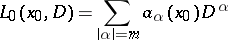
One of the methods for studying boundary value problems for differential equations with variable coefficients by means of integral equations.
Suppose that in some region  of the
  -dimensional Euclidean space
  one considers an elliptic differential operator (cf. Elliptic partial differential equation) of order
  ,
,
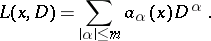 | (1) |
In (1) the symbol  is a multi-index,
  , where the
  are non-negative integers,
  ,
,  ,
,  . With every operator (1) there is associated the homogeneous elliptic operator
 |
with constant coefficients, where  is an arbitrary fixed point. Let
  denote a fundamental solution of
  depending parametrically on
  . Then the function
  is called the parametrix of the operator (1) with a singularity at
  .
.
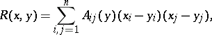
In particular, for the second-order elliptic operator
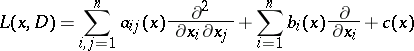 |
one can take as parametrix with singularity at  the Levi function
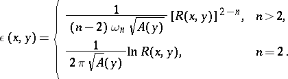 | (2) |
In (2), 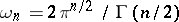 ,
,  is the determinant of the matrix
  ,
,
 |
and  are the elements of the matrix inverse to
  .
.
Let  be the integral operator
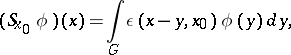 | (3) |
acting on functions from  and let
 |
Since, by definition of a fundamental solution,
 |
where  is the identity operator, one has
 |
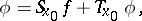
This equality indicates that for every sufficiently-smooth function  of compact support in
  there is a representation
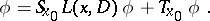 | (4) |
Moreover, if
 |
then  is a solution of the equation
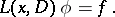 |
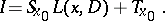
Thus, the question of the local solvability of  reduces to that of invertibility of
  .
.
If one applies  to functions
  that vanish outside a ball of radius
  with centre at
  , then for a sufficiently small
  the norm of
  can be made smaller than one. Then the operator
  exists; consequently, also
 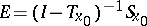 exists, which is the inverse operator to
  . Here
  is an integral operator with as kernel a fundamental solution of
  .
.
The name parametrix is sometimes given not only to the function  , but also to the integral operator
  with the kernel
  , as defined by (3).
In the theory of pseudo-differential operators, instead of  a parametrix of
  is defined as an operator
  such that
  and
and  are integral operators with infinitely-differentiable kernels (cf. Pseudo-differential operator). If only
  (or
(or  ) is such an operator, then
  is called a left (or right) parametrix of
  . In other words,
  in (4) is a left parametrix if
  in this equality has an infinitely-differentiable kernel. If
  has a left parametrix
  and a right parametrix
  , then each of them is a parametrix. The existence of a parametrix has been proved for hypo-elliptic pseudo-differential operators (see [3]).
References
| [1] | L. Bers, F. John, M. Schechter, "Partial differential equations" , Interscience (1964) |
| [2] | C. Miranda, "Partial differential equations of elliptic type" , Springer (1970) (Translated from Italian) |
| [3] | L. Hörmander, , Pseudo-differential operators , Moscow (1967) (In Russian; translated from English) |
Comments
The operator  is called the principal part of
  , cf. Principal part of a differential operator. The parametrix method was anticipated in two fundamental papers by E.E. Levi [a1], [a2]. The same procedure is also applicable for constructing the fundamental solution of a parabolic equation with variable coefficients (see, e.g., [a3]).
References
| [a1] | E.E. Levi, "Sulle equazioni lineari alle derivate parziali totalmente ellittiche" Rend. R. Acc. Lincei, Classe Sci. (V) , 16 (1907) |
| [a2] | E.E. Levi, "Sulle equazioni lineari totalmente ellittiche alle derivate parziali" Rend. Circ. Mat. Palermo , 24 (1907) pp. 275–317 |
| [a3] | A. Friedman, "Partial differential equations of parabolic type" , Prentice-Hall (1964) |
| [a4] | L.V. Hörmander, "The analysis of linear partial differential operators" , 1–4 , Springer (1983–1985) pp. Chapts. 7; 18 |
Parametrix method. Encyclopedia of Mathematics. URL: http://encyclopediaofmath.org/index.php?title=Parametrix_method&oldid=49355