Difference between revisions of "Parametric resonance, mathematical theory of"
Ulf Rehmann (talk | contribs) m (tex encoded by computer) |
Ulf Rehmann (talk | contribs) m (Undo revision 48128 by Ulf Rehmann (talk)) Tag: Undo |
||
| Line 1: | Line 1: | ||
| − | |||
| − | |||
| − | |||
| − | |||
| − | |||
| − | |||
| − | |||
| − | |||
| − | |||
| − | |||
| − | |||
| − | |||
The branch of the theory of ordinary differential equations that studies the phenomenon of parametric resonance. | The branch of the theory of ordinary differential equations that studies the phenomenon of parametric resonance. | ||
| − | Let | + | Let <img align="absmiddle" border="0" src="https://www.encyclopediaofmath.org/legacyimages/p/p071/p071560/p0715601.png" /> be a dynamical system that can only perform oscillatory motions and that is given by a linear Hamiltonian system (cf. [[Hamiltonian system, linear|Hamiltonian system, linear]]) (an unperturbed equation) |
| − | be a dynamical system that can only perform oscillatory motions and that is given by a linear Hamiltonian system (cf. [[Hamiltonian system, linear|Hamiltonian system, linear]]) (an unperturbed equation) | ||
| − | + | <table class="eq" style="width:100%;"> <tr><td valign="top" style="width:94%;text-align:center;"><img align="absmiddle" border="0" src="https://www.encyclopediaofmath.org/legacyimages/p/p071/p071560/p0715602.png" /></td> </tr></table> | |
| − | |||
| − | |||
| − | with a constant real positive Hamiltonian | + | with a constant real positive Hamiltonian <img align="absmiddle" border="0" src="https://www.encyclopediaofmath.org/legacyimages/p/p071/p071560/p0715603.png" />. Thus, the <img align="absmiddle" border="0" src="https://www.encyclopediaofmath.org/legacyimages/p/p071/p071560/p0715604.png" />-matrix <img align="absmiddle" border="0" src="https://www.encyclopediaofmath.org/legacyimages/p/p071/p071560/p0715605.png" /> can be brought to diagonal form with purely-imaginary elements |
| − | Thus, the | ||
| − | matrix | ||
| − | can be brought to diagonal form with purely-imaginary elements | ||
| − | + | <table class="eq" style="width:100%;"> <tr><td valign="top" style="width:94%;text-align:center;"><img align="absmiddle" border="0" src="https://www.encyclopediaofmath.org/legacyimages/p/p071/p071560/p0715606.png" /></td> </tr></table> | |
| − | |||
| − | |||
| − | |||
| − | |||
| − | the | + | the <img align="absmiddle" border="0" src="https://www.encyclopediaofmath.org/legacyimages/p/p071/p071560/p0715607.png" /> being the eigen frequencies of the system. Suppose that some parameters of <img align="absmiddle" border="0" src="https://www.encyclopediaofmath.org/legacyimages/p/p071/p071560/p0715608.png" /> begin to change periodically with a frequency <img align="absmiddle" border="0" src="https://www.encyclopediaofmath.org/legacyimages/p/p071/p071560/p0715609.png" /> and with small amplitudes the values of which are determined by a small parameter <img align="absmiddle" border="0" src="https://www.encyclopediaofmath.org/legacyimages/p/p071/p071560/p07156010.png" />. If the perturbation does not lead out of the class of linear Hamiltonian systems, then the motion of <img align="absmiddle" border="0" src="https://www.encyclopediaofmath.org/legacyimages/p/p071/p071560/p07156011.png" /> can be described by the perturbed equation |
| − | being the eigen frequencies of the system. Suppose that some parameters of | ||
| − | begin to change periodically with a frequency | ||
| − | and with small amplitudes the values of which are determined by a small parameter | ||
| − | If the perturbation does not lead out of the class of linear Hamiltonian systems, then the motion of | ||
| − | can be described by the perturbed equation | ||
| − | + | <table class="eq" style="width:100%;"> <tr><td valign="top" style="width:94%;text-align:center;"><img align="absmiddle" border="0" src="https://www.encyclopediaofmath.org/legacyimages/p/p071/p071560/p07156012.png" /></td> <td valign="top" style="width:5%;text-align:right;">(1)</td></tr></table> | |
| − | |||
| − | |||
| − | |||
| − | where the | + | where the <img align="absmiddle" border="0" src="https://www.encyclopediaofmath.org/legacyimages/p/p071/p071560/p07156013.png" />, <img align="absmiddle" border="0" src="https://www.encyclopediaofmath.org/legacyimages/p/p071/p071560/p07156014.png" /> are piecewise-continuous <img align="absmiddle" border="0" src="https://www.encyclopediaofmath.org/legacyimages/p/p071/p071560/p07156015.png" />-matrix-valued functions, integrable on <img align="absmiddle" border="0" src="https://www.encyclopediaofmath.org/legacyimages/p/p071/p071560/p07156016.png" />, and where the series on the right-hand side of (1) converges for <img align="absmiddle" border="0" src="https://www.encyclopediaofmath.org/legacyimages/p/p071/p071560/p07156017.png" />, <img align="absmiddle" border="0" src="https://www.encyclopediaofmath.org/legacyimages/p/p071/p071560/p07156018.png" /> being independent of <img align="absmiddle" border="0" src="https://www.encyclopediaofmath.org/legacyimages/p/p071/p071560/p07156019.png" />. |
| − | |||
| − | are piecewise-continuous | ||
| − | matrix-valued functions, integrable on | ||
| − | and where the series on the right-hand side of (1) converges for | ||
| − | |||
| − | being independent of | ||
| − | The emergence of unboundedly-increasing oscillations of | + | The emergence of unboundedly-increasing oscillations of <img align="absmiddle" border="0" src="https://www.encyclopediaofmath.org/legacyimages/p/p071/p071560/p07156020.png" /> under an arbitrarily small periodic perturbation of its parameters is called parametric resonance. It has two essential peculiarities: 1) the spectrum of frequencies for which there arise unboundedly-increasing oscillations is not a point spectrum but consists of a collection of small intervals with lengths depending on the amplitude of the perturbations (that is, on <img align="absmiddle" border="0" src="https://www.encyclopediaofmath.org/legacyimages/p/p071/p071560/p07156021.png" />) and contracting to a point as <img align="absmiddle" border="0" src="https://www.encyclopediaofmath.org/legacyimages/p/p071/p071560/p07156022.png" />; the values of the frequencies to which these intervals contract are called critical; 2) the oscillations grow not by a power but by an exponential law. This parametric resonance is considerably more "dangerous" (or "useful" , depending on the problem) than ordinary resonance. |
| − | under an arbitrarily small periodic perturbation of its parameters is called parametric resonance. It has two essential peculiarities: 1) the spectrum of frequencies for which there arise unboundedly-increasing oscillations is not a point spectrum but consists of a collection of small intervals with lengths depending on the amplitude of the perturbations (that is, on | ||
| − | and contracting to a point as | ||
| − | the values of the frequencies to which these intervals contract are called critical; 2) the oscillations grow not by a power but by an exponential law. This parametric resonance is considerably more "dangerous" (or "useful" , depending on the problem) than ordinary resonance. | ||
| − | Let | + | Let <img align="absmiddle" border="0" src="https://www.encyclopediaofmath.org/legacyimages/p/p071/p071560/p07156023.png" /> be the eigen values of the first kind, numbered so that <img align="absmiddle" border="0" src="https://www.encyclopediaofmath.org/legacyimages/p/p071/p071560/p07156024.png" />. Then only frequencies of the following form can be critical: |
| − | be the eigen values of the first kind, numbered so that | ||
| − | Then only frequencies of the following form can be critical: | ||
| − | + | <table class="eq" style="width:100%;"> <tr><td valign="top" style="width:94%;text-align:center;"><img align="absmiddle" border="0" src="https://www.encyclopediaofmath.org/legacyimages/p/p071/p071560/p07156025.png" /></td> <td valign="top" style="width:5%;text-align:right;">(2)</td></tr></table> | |
| − | |||
| − | |||
| − | |||
| − | |||
| − | |||
| − | |||
| − | Suppose that the eigen vectors | + | Suppose that the eigen vectors <img align="absmiddle" border="0" src="https://www.encyclopediaofmath.org/legacyimages/p/p071/p071560/p07156026.png" /> of <img align="absmiddle" border="0" src="https://www.encyclopediaofmath.org/legacyimages/p/p071/p071560/p07156027.png" /> for which <img align="absmiddle" border="0" src="https://www.encyclopediaofmath.org/legacyimages/p/p071/p071560/p07156028.png" />, <img align="absmiddle" border="0" src="https://www.encyclopediaofmath.org/legacyimages/p/p071/p071560/p07156029.png" />, are normalized so that |
| − | of | ||
| − | for which | ||
| − | |||
| − | are normalized so that | ||
| − | + | <table class="eq" style="width:100%;"> <tr><td valign="top" style="width:94%;text-align:center;"><img align="absmiddle" border="0" src="https://www.encyclopediaofmath.org/legacyimages/p/p071/p071560/p07156030.png" /></td> </tr></table> | |
| − | |||
| − | |||
| − | |||
| − | where | + | where <img align="absmiddle" border="0" src="https://www.encyclopediaofmath.org/legacyimages/p/p071/p071560/p07156031.png" /> is the Kronecker symbol and |
| − | is the Kronecker symbol and | ||
| − | + | <table class="eq" style="width:100%;"> <tr><td valign="top" style="width:94%;text-align:center;"><img align="absmiddle" border="0" src="https://www.encyclopediaofmath.org/legacyimages/p/p071/p071560/p07156032.png" /></td> </tr></table> | |
| − | |||
| − | |||
| − | Then the domains of instability in a first approximation in | + | Then the domains of instability in a first approximation in <img align="absmiddle" border="0" src="https://www.encyclopediaofmath.org/legacyimages/p/p071/p071560/p07156033.png" /> are determined by the inequalities |
| − | are determined by the inequalities | ||
| − | + | <table class="eq" style="width:100%;"> <tr><td valign="top" style="width:94%;text-align:center;"><img align="absmiddle" border="0" src="https://www.encyclopediaofmath.org/legacyimages/p/p071/p071560/p07156034.png" /></td> <td valign="top" style="width:5%;text-align:right;">(3)</td></tr></table> | |
| − | |||
| − | |||
where | where | ||
| − | + | <table class="eq" style="width:100%;"> <tr><td valign="top" style="width:94%;text-align:center;"><img align="absmiddle" border="0" src="https://www.encyclopediaofmath.org/legacyimages/p/p071/p071560/p07156035.png" /></td> <td valign="top" style="width:5%;text-align:right;">(4)</td></tr></table> | |
| − | |||
| − | |||
| − | If | + | If <img align="absmiddle" border="0" src="https://www.encyclopediaofmath.org/legacyimages/p/p071/p071560/p07156036.png" />, then the domain of instability corresponds to a basic resonance, and for <img align="absmiddle" border="0" src="https://www.encyclopediaofmath.org/legacyimages/p/p071/p071560/p07156037.png" /> to a combined resonance. The quantities <img align="absmiddle" border="0" src="https://www.encyclopediaofmath.org/legacyimages/p/p071/p071560/p07156038.png" /> characterize the "degree of danger" of the critical frequency <img align="absmiddle" border="0" src="https://www.encyclopediaofmath.org/legacyimages/p/p071/p071560/p07156039.png" />: the larger this quantity, the wider is the "wedge" of instability (3), with a peak at <img align="absmiddle" border="0" src="https://www.encyclopediaofmath.org/legacyimages/p/p071/p071560/p07156040.png" />. The analytic dependence on the parameter <img align="absmiddle" border="0" src="https://www.encyclopediaofmath.org/legacyimages/p/p071/p071560/p07156041.png" /> of the boundaries of the domains of instability has been established and effective formulas have been obtained for the computation of the domains (3) in the second approximation (see [[#References|[3]]], [[#References|[4]]], [[#References|[9]]]). |
| − | then the domain of instability corresponds to a basic resonance, and for | ||
| − | to a combined resonance. The quantities | ||
| − | characterize the "degree of danger" of the critical frequency | ||
| − | the larger this quantity, the wider is the "wedge" of instability (3), with a peak at | ||
| − | The analytic dependence on the parameter | ||
| − | of the boundaries of the domains of instability has been established and effective formulas have been obtained for the computation of the domains (3) in the second approximation (see [[#References|[3]]], [[#References|[4]]], [[#References|[9]]]). | ||
| − | In the case, frequently occurring in applications, when the perturbed system | + | In the case, frequently occurring in applications, when the perturbed system <img align="absmiddle" border="0" src="https://www.encyclopediaofmath.org/legacyimages/p/p071/p071560/p07156042.png" /> can be described by a second-order vector-valued equation |
| − | can be described by a second-order vector-valued equation | ||
| − | + | <table class="eq" style="width:100%;"> <tr><td valign="top" style="width:94%;text-align:center;"><img align="absmiddle" border="0" src="https://www.encyclopediaofmath.org/legacyimages/p/p071/p071560/p07156043.png" /></td> <td valign="top" style="width:5%;text-align:right;">(5)</td></tr></table> | |
| − | |||
| − | |||
| − | |||
| − | where | + | where <img align="absmiddle" border="0" src="https://www.encyclopediaofmath.org/legacyimages/p/p071/p071560/p07156044.png" /> and <img align="absmiddle" border="0" src="https://www.encyclopediaofmath.org/legacyimages/p/p071/p071560/p07156045.png" />, <img align="absmiddle" border="0" src="https://www.encyclopediaofmath.org/legacyimages/p/p071/p071560/p07156046.png" /> the eigen vectors and eigen values of <img align="absmiddle" border="0" src="https://www.encyclopediaofmath.org/legacyimages/p/p071/p071560/p07156047.png" /> (the squares of the frequencies of the undisturbed system) are determined by |
| − | and | ||
| − | |||
| − | the eigen vectors and eigen values of | ||
| − | the squares of the frequencies of the undisturbed system) are determined by | ||
| − | + | <table class="eq" style="width:100%;"> <tr><td valign="top" style="width:94%;text-align:center;"><img align="absmiddle" border="0" src="https://www.encyclopediaofmath.org/legacyimages/p/p071/p071560/p07156048.png" /></td> </tr></table> | |
| − | |||
| − | |||
| − | + | <table class="eq" style="width:100%;"> <tr><td valign="top" style="width:94%;text-align:center;"><img align="absmiddle" border="0" src="https://www.encyclopediaofmath.org/legacyimages/p/p071/p071560/p07156049.png" /></td> </tr></table> | |
| − | |||
| − | |||
| − | |||
Let | Let | ||
| − | + | <table class="eq" style="width:100%;"> <tr><td valign="top" style="width:94%;text-align:center;"><img align="absmiddle" border="0" src="https://www.encyclopediaofmath.org/legacyimages/p/p071/p071560/p07156050.png" /></td> </tr></table> | |
| − | |||
| − | |||
Then (2) and (4) take the form | Then (2) and (4) take the form | ||
| − | + | <table class="eq" style="width:100%;"> <tr><td valign="top" style="width:94%;text-align:center;"><img align="absmiddle" border="0" src="https://www.encyclopediaofmath.org/legacyimages/p/p071/p071560/p07156051.png" /></td> </tr></table> | |
| − | |||
| − | |||
| − | |||
| − | |||
| − | |||
| − | + | <table class="eq" style="width:100%;"> <tr><td valign="top" style="width:94%;text-align:center;"><img align="absmiddle" border="0" src="https://www.encyclopediaofmath.org/legacyimages/p/p071/p071560/p07156052.png" /></td> </tr></table> | |
| − | |||
| − | |||
| − | respectively. In particular, in a basis | + | respectively. In particular, in a basis <img align="absmiddle" border="0" src="https://www.encyclopediaofmath.org/legacyimages/p/p071/p071560/p07156053.png" /> in which <img align="absmiddle" border="0" src="https://www.encyclopediaofmath.org/legacyimages/p/p071/p071560/p07156054.png" /> is in diagonal form: |
| − | in which | ||
| − | is in diagonal form: | ||
| − | + | <table class="eq" style="width:100%;"> <tr><td valign="top" style="width:94%;text-align:center;"><img align="absmiddle" border="0" src="https://www.encyclopediaofmath.org/legacyimages/p/p071/p071560/p07156055.png" /></td> </tr></table> | |
| − | |||
| − | |||
and | and | ||
| − | + | <table class="eq" style="width:100%;"> <tr><td valign="top" style="width:94%;text-align:center;"><img align="absmiddle" border="0" src="https://www.encyclopediaofmath.org/legacyimages/p/p071/p071560/p07156056.png" /></td> </tr></table> | |
| − | |||
| − | |||
| − | |||
one has | one has | ||
| − | + | <table class="eq" style="width:100%;"> <tr><td valign="top" style="width:94%;text-align:center;"><img align="absmiddle" border="0" src="https://www.encyclopediaofmath.org/legacyimages/p/p071/p071560/p07156057.png" /></td> </tr></table> | |
| − | |||
| − | |||
| − | |||
| − | |||
| − | |||
| − | |||
and consequently (see [[#References|[5]]]) | and consequently (see [[#References|[5]]]) | ||
| − | + | <table class="eq" style="width:100%;"> <tr><td valign="top" style="width:94%;text-align:center;"><img align="absmiddle" border="0" src="https://www.encyclopediaofmath.org/legacyimages/p/p071/p071560/p07156058.png" /></td> </tr></table> | |
| − | |||
| − | |||
| − | |||
| − | |||
| − | |||
| − | |||
| − | |||
| − | + | <table class="eq" style="width:100%;"> <tr><td valign="top" style="width:94%;text-align:center;"><img align="absmiddle" border="0" src="https://www.encyclopediaofmath.org/legacyimages/p/p071/p071560/p07156059.png" /></td> </tr></table> | |
| − | |||
| − | |||
| − | |||
| − | |||
| − | The case of a non-linear dependence of the coefficients of (1) and (5) on the parameter | + | The case of a non-linear dependence of the coefficients of (1) and (5) on the parameter <img align="absmiddle" border="0" src="https://www.encyclopediaofmath.org/legacyimages/p/p071/p071560/p07156060.png" /> has also been treated (see [[#References|[4]]], [[#References|[9]]]). Parametric resonance in linear systems close to being Hamiltonian has been studied (see [[#References|[6]]], [[#References|[9]]]). Here the domains of basic resonance form those of principal resonance, and together with the domains of combined resonance there appear domains of combined-difference resonance. For parametric resonance in linear distributed systems (see [[#References|[7]]]) a number of similar results have been obtained for operator equations (1) in a Hilbert space. Parametric resonance has also been investigated for certain classes of systems with finitely many degrees of freedom that can be described by non-linear differential equations (see [[#References|[8]]]). |
| − | has also been treated (see [[#References|[4]]], [[#References|[9]]]). Parametric resonance in linear systems close to being Hamiltonian has been studied (see [[#References|[6]]], [[#References|[9]]]). Here the domains of basic resonance form those of principal resonance, and together with the domains of combined resonance there appear domains of combined-difference resonance. For parametric resonance in linear distributed systems (see [[#References|[7]]]) a number of similar results have been obtained for operator equations (1) in a Hilbert space. Parametric resonance has also been investigated for certain classes of systems with finitely many degrees of freedom that can be described by non-linear differential equations (see [[#References|[8]]]). | ||
====References==== | ====References==== | ||
<table><TR><TD valign="top">[1]</TD> <TD valign="top"> M.G. Krein, "Foundations of the theory of <img align="absmiddle" border="0" src="https://www.encyclopediaofmath.org/legacyimages/p/p071/p071560/p07156061.png" />-zones of stability of a canonical system of linear differential equations with periodic coefficients" ''Transl. Amer. Math. Soc. (2)'' , '''120''' (1983) pp. 1–70 ''In memoriam: A.A. Andronov'' (1955) pp. 413–498</TD></TR><TR><TD valign="top">[2]</TD> <TD valign="top"> V.A. Yakubovich, "On the dynamic stability of elastic systems" ''Dokl. Akad. Nauk SSSR'' , '''121''' : 4 (1958) pp. 602–605 (In Russian)</TD></TR><TR><TD valign="top">[3]</TD> <TD valign="top"> V.A. Yakubovich, "Regions of dynamic instability of Hamiltonian systems" ''Metody Vychisl.'' , '''3''' (1966) pp. 51–69 (In Russian)</TD></TR><TR><TD valign="top">[4]</TD> <TD valign="top"> V.A. Yakubovich, V.M. Starzhinskii, "Linear differential equations with periodic coefficients and their applications" , '''1–2''' , Wiley (1975) (Translated from Russian)</TD></TR><TR><TD valign="top">[5]</TD> <TD valign="top"> I.G. Malkin, "Some problems in the theory of non-linear oscillations" , Moscow (1956) (In Russian)</TD></TR><TR><TD valign="top">[6]</TD> <TD valign="top"> V.M. Starzhinskii, ''Inzh. Zh. Mekh. Tverd. Tela'' , '''3''' (1967) pp. 174–180</TD></TR><TR><TD valign="top">[7]</TD> <TD valign="top"> V.N. Fomin, "Mathematical theory of parameter resonance in linear distributed systems" , Leningrad (1972) (In Russian)</TD></TR><TR><TD valign="top">[8]</TD> <TD valign="top"> G. Schmidt, "Parametererregte Schwingungen" , Deutsch. Verlag Wissenschaft. (1975)</TD></TR><TR><TD valign="top">[9]</TD> <TD valign="top"> V.A. Yakubovich, V.M. Starzhinskii, "Parameter resonance in linear systems" , Moscow (1987) (In Russian)</TD></TR></table> | <table><TR><TD valign="top">[1]</TD> <TD valign="top"> M.G. Krein, "Foundations of the theory of <img align="absmiddle" border="0" src="https://www.encyclopediaofmath.org/legacyimages/p/p071/p071560/p07156061.png" />-zones of stability of a canonical system of linear differential equations with periodic coefficients" ''Transl. Amer. Math. Soc. (2)'' , '''120''' (1983) pp. 1–70 ''In memoriam: A.A. Andronov'' (1955) pp. 413–498</TD></TR><TR><TD valign="top">[2]</TD> <TD valign="top"> V.A. Yakubovich, "On the dynamic stability of elastic systems" ''Dokl. Akad. Nauk SSSR'' , '''121''' : 4 (1958) pp. 602–605 (In Russian)</TD></TR><TR><TD valign="top">[3]</TD> <TD valign="top"> V.A. Yakubovich, "Regions of dynamic instability of Hamiltonian systems" ''Metody Vychisl.'' , '''3''' (1966) pp. 51–69 (In Russian)</TD></TR><TR><TD valign="top">[4]</TD> <TD valign="top"> V.A. Yakubovich, V.M. Starzhinskii, "Linear differential equations with periodic coefficients and their applications" , '''1–2''' , Wiley (1975) (Translated from Russian)</TD></TR><TR><TD valign="top">[5]</TD> <TD valign="top"> I.G. Malkin, "Some problems in the theory of non-linear oscillations" , Moscow (1956) (In Russian)</TD></TR><TR><TD valign="top">[6]</TD> <TD valign="top"> V.M. Starzhinskii, ''Inzh. Zh. Mekh. Tverd. Tela'' , '''3''' (1967) pp. 174–180</TD></TR><TR><TD valign="top">[7]</TD> <TD valign="top"> V.N. Fomin, "Mathematical theory of parameter resonance in linear distributed systems" , Leningrad (1972) (In Russian)</TD></TR><TR><TD valign="top">[8]</TD> <TD valign="top"> G. Schmidt, "Parametererregte Schwingungen" , Deutsch. Verlag Wissenschaft. (1975)</TD></TR><TR><TD valign="top">[9]</TD> <TD valign="top"> V.A. Yakubovich, V.M. Starzhinskii, "Parameter resonance in linear systems" , Moscow (1987) (In Russian)</TD></TR></table> | ||
| + | |||
| + | |||
====Comments==== | ====Comments==== | ||
Revision as of 14:52, 7 June 2020
The branch of the theory of ordinary differential equations that studies the phenomenon of parametric resonance.
Let  be a dynamical system that can only perform oscillatory motions and that is given by a linear Hamiltonian system (cf. Hamiltonian system, linear) (an unperturbed equation)
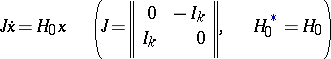 |
with a constant real positive Hamiltonian  . Thus, the
  -matrix
  can be brought to diagonal form with purely-imaginary elements
 |
the  being the eigen frequencies of the system. Suppose that some parameters of
  begin to change periodically with a frequency
  and with small amplitudes the values of which are determined by a small parameter
  . If the perturbation does not lead out of the class of linear Hamiltonian systems, then the motion of
  can be described by the perturbed equation
 | (1) |
where the 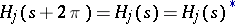 ,
,  are piecewise-continuous
  -matrix-valued functions, integrable on
  , and where the series on the right-hand side of (1) converges for
  ,
,  being independent of
  .
.
The emergence of unboundedly-increasing oscillations of  under an arbitrarily small periodic perturbation of its parameters is called parametric resonance. It has two essential peculiarities: 1) the spectrum of frequencies for which there arise unboundedly-increasing oscillations is not a point spectrum but consists of a collection of small intervals with lengths depending on the amplitude of the perturbations (that is, on
  ) and contracting to a point as
  ; the values of the frequencies to which these intervals contract are called critical; 2) the oscillations grow not by a power but by an exponential law. This parametric resonance is considerably more "dangerous" (or "useful" , depending on the problem) than ordinary resonance.
Let  be the eigen values of the first kind, numbered so that
 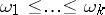 . Then only frequencies of the following form can be critical:
 | (2) |
Suppose that the eigen vectors  of
of  for which
 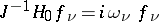 ,
,  , are normalized so that
 |
where  is the Kronecker symbol and
 |
Then the domains of instability in a first approximation in  are determined by the inequalities
 | (3) |
where
 | (4) |
If  , then the domain of instability corresponds to a basic resonance, and for
  to a combined resonance. The quantities
  characterize the "degree of danger" of the critical frequency
  : the larger this quantity, the wider is the "wedge" of instability (3), with a peak at
  . The analytic dependence on the parameter
  of the boundaries of the domains of instability has been established and effective formulas have been obtained for the computation of the domains (3) in the second approximation (see [3], [4], [9]).
In the case, frequently occurring in applications, when the perturbed system  can be described by a second-order vector-valued equation
 | (5) |
where  and
and  ,
,  the eigen vectors and eigen values of
  (the squares of the frequencies of the undisturbed system) are determined by
 |
 |
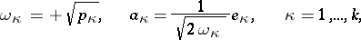
Let
 |
Then (2) and (4) take the form
 |
 |
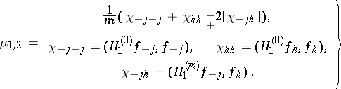
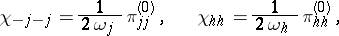
respectively. In particular, in a basis  in which
  is in diagonal form:
 |
and
 |
one has
 |
and consequently (see [5])
 |
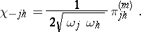 |
The case of a non-linear dependence of the coefficients of (1) and (5) on the parameter  has also been treated (see [4], [9]). Parametric resonance in linear systems close to being Hamiltonian has been studied (see [6], [9]). Here the domains of basic resonance form those of principal resonance, and together with the domains of combined resonance there appear domains of combined-difference resonance. For parametric resonance in linear distributed systems (see [7]) a number of similar results have been obtained for operator equations (1) in a Hilbert space. Parametric resonance has also been investigated for certain classes of systems with finitely many degrees of freedom that can be described by non-linear differential equations (see [8]).
References
| [1] | M.G. Krein, "Foundations of the theory of  -zones of stability of a canonical system of linear differential equations with periodic coefficients" Transl. Amer. Math. Soc. (2) , 120 (1983) pp. 1–70 In memoriam: A.A. Andronov (1955) pp. 413–498 -zones of stability of a canonical system of linear differential equations with periodic coefficients" Transl. Amer. Math. Soc. (2) , 120 (1983) pp. 1–70 In memoriam: A.A. Andronov (1955) pp. 413–498 |
| [2] | V.A. Yakubovich, "On the dynamic stability of elastic systems" Dokl. Akad. Nauk SSSR , 121 : 4 (1958) pp. 602–605 (In Russian) |
| [3] | V.A. Yakubovich, "Regions of dynamic instability of Hamiltonian systems" Metody Vychisl. , 3 (1966) pp. 51–69 (In Russian) |
| [4] | V.A. Yakubovich, V.M. Starzhinskii, "Linear differential equations with periodic coefficients and their applications" , 1–2 , Wiley (1975) (Translated from Russian) |
| [5] | I.G. Malkin, "Some problems in the theory of non-linear oscillations" , Moscow (1956) (In Russian) |
| [6] | V.M. Starzhinskii, Inzh. Zh. Mekh. Tverd. Tela , 3 (1967) pp. 174–180 |
| [7] | V.N. Fomin, "Mathematical theory of parameter resonance in linear distributed systems" , Leningrad (1972) (In Russian) |
| [8] | G. Schmidt, "Parametererregte Schwingungen" , Deutsch. Verlag Wissenschaft. (1975) |
| [9] | V.A. Yakubovich, V.M. Starzhinskii, "Parameter resonance in linear systems" , Moscow (1987) (In Russian) |
Comments
Parametric resonances, or parametrically sustained vibrations, naturally occur e.g. in electric wires and pantographs (devices for reproducing motions or geometric drawings at an enlarged or reduced scale) and care must be taken in the design to control them. On the other hand, various parametric devices in electronics (for instance, a parametric amplifier) make effective use of parametric resonances.
References
| [a1] | V.I. Arnol'd, A. Avez, "Problèmes ergodiques de la mécanique classique" , Gauthier-Villars (1967) pp. §20.5; Append. 29 (Translated from Russian) |
Parametric resonance, mathematical theory of. Encyclopedia of Mathematics. URL: http://encyclopediaofmath.org/index.php?title=Parametric_resonance,_mathematical_theory_of&oldid=49354