Difference between revisions of "Optimal sliding regime"
Ulf Rehmann (talk | contribs) m (tex encoded by computer) |
Ulf Rehmann (talk | contribs) m (Undo revision 48056 by Ulf Rehmann (talk)) Tag: Undo |
||
| Line 1: | Line 1: | ||
| − | |||
| − | |||
| − | |||
| − | |||
| − | |||
| − | |||
| − | |||
| − | |||
| − | |||
| − | |||
| − | |||
| − | |||
A term used in the theory of [[Optimal control|optimal control]] to describe an optimal method of controlling a system when a minimizing sequence of control functions does not have a limit in the class of Lebesgue-measurable functions. | A term used in the theory of [[Optimal control|optimal control]] to describe an optimal method of controlling a system when a minimizing sequence of control functions does not have a limit in the class of Lebesgue-measurable functions. | ||
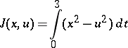
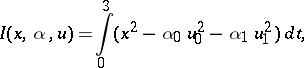
For example, suppose a minimum of the functional | For example, suppose a minimum of the functional | ||
| − | + | <table class="eq" style="width:100%;"> <tr><td valign="top" style="width:94%;text-align:center;"><img align="absmiddle" border="0" src="https://www.encyclopediaofmath.org/legacyimages/o/o068/o068490/o0684901.png" /></td> <td valign="top" style="width:5%;text-align:right;">(1)</td></tr></table> | |
| − | |||
| − | |||
has to be found, given the constraints | has to be found, given the constraints | ||
| − | + | <table class="eq" style="width:100%;"> <tr><td valign="top" style="width:94%;text-align:center;"><img align="absmiddle" border="0" src="https://www.encyclopediaofmath.org/legacyimages/o/o068/o068490/o0684902.png" /></td> <td valign="top" style="width:5%;text-align:right;">(2)</td></tr></table> | |
| − | |||
| − | |||
| − | |||
| − | |||
| − | |||
| − | |||
| − | |||
| − | |||
| − | |||
| − | |||
| − | + | <table class="eq" style="width:100%;"> <tr><td valign="top" style="width:94%;text-align:center;"><img align="absmiddle" border="0" src="https://www.encyclopediaofmath.org/legacyimages/o/o068/o068490/o0684903.png" /></td> <td valign="top" style="width:5%;text-align:right;">(3)</td></tr></table> | |
| − | |||
| − | |||
| − | |||
| − | + | <table class="eq" style="width:100%;"> <tr><td valign="top" style="width:94%;text-align:center;"><img align="absmiddle" border="0" src="https://www.encyclopediaofmath.org/legacyimages/o/o068/o068490/o0684904.png" /></td> <td valign="top" style="width:5%;text-align:right;">(4)</td></tr></table> | |
| − | |||
| − | |||
| − | |||
| − | |||
| − | |||
| − | |||
| − | + | In order to obtain a minimum of the functional (1), it is desirable for every <img align="absmiddle" border="0" src="https://www.encyclopediaofmath.org/legacyimages/o/o068/o068490/o0684905.png" /> to have as small a value as possible of <img align="absmiddle" border="0" src="https://www.encyclopediaofmath.org/legacyimages/o/o068/o068490/o0684906.png" /> and as large a value as possible of <img align="absmiddle" border="0" src="https://www.encyclopediaofmath.org/legacyimages/o/o068/o068490/o0684907.png" />. The first requirement, with regard to the constraining condition (2), the boundary conditions (3) and the control constraint (4), is satisfied by the trajectory | |
| − | |||
| − | |||
| − | |||
| − | |||
| − | |||
| − | + | <table class="eq" style="width:100%;"> <tr><td valign="top" style="width:94%;text-align:center;"><img align="absmiddle" border="0" src="https://www.encyclopediaofmath.org/legacyimages/o/o068/o068490/o0684908.png" /></td> <td valign="top" style="width:5%;text-align:right;">(5)</td></tr></table> | |
| − | If the trajectory (5) could be created for a control which, for all | + | If the trajectory (5) could be created for a control which, for all <img align="absmiddle" border="0" src="https://www.encyclopediaofmath.org/legacyimages/o/o068/o068490/o0684909.png" />, has the boundary values |
| − | has the boundary values | ||
| − | + | <table class="eq" style="width:100%;"> <tr><td valign="top" style="width:94%;text-align:center;"><img align="absmiddle" border="0" src="https://www.encyclopediaofmath.org/legacyimages/o/o068/o068490/o06849010.png" /></td> <td valign="top" style="width:5%;text-align:right;">(6)</td></tr></table> | |
| − | |||
| − | |||
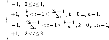
| − | the absolute minimum of the functional (1) would be obtained. However, the "ideal" trajectory (5) cannot be created for any control function | + | the absolute minimum of the functional (1) would be obtained. However, the "ideal" trajectory (5) cannot be created for any control function <img align="absmiddle" border="0" src="https://www.encyclopediaofmath.org/legacyimages/o/o068/o068490/o06849011.png" /> which satisfies (6), since, when <img align="absmiddle" border="0" src="https://www.encyclopediaofmath.org/legacyimages/o/o068/o068490/o06849012.png" />, <img align="absmiddle" border="0" src="https://www.encyclopediaofmath.org/legacyimages/o/o068/o068490/o06849013.png" />. Nevertheless, it is possible, using control functions <img align="absmiddle" border="0" src="https://www.encyclopediaofmath.org/legacyimages/o/o068/o068490/o06849014.png" /> which, when <img align="absmiddle" border="0" src="https://www.encyclopediaofmath.org/legacyimages/o/o068/o068490/o06849015.png" /> and <img align="absmiddle" border="0" src="https://www.encyclopediaofmath.org/legacyimages/o/o068/o068490/o06849016.png" />, realize ever more frequent switchings from 1 to <img align="absmiddle" border="0" src="https://www.encyclopediaofmath.org/legacyimages/o/o068/o068490/o06849017.png" /> and vice versa: |
| − | which satisfies (6), since, when | ||
| − | |||
| − | Nevertheless, it is possible, using control functions | ||
| − | which, when | ||
| − | and | ||
| − | realize ever more frequent switchings from 1 to | ||
| − | and vice versa: | ||
| − | + | <table class="eq" style="width:100%;"> <tr><td valign="top" style="width:94%;text-align:center;"><img align="absmiddle" border="0" src="https://www.encyclopediaofmath.org/legacyimages/o/o068/o068490/o06849018.png" /></td> <td valign="top" style="width:5%;text-align:right;">(7)</td></tr></table> | |
| − | |||
| − | |||
| − | + | <table class="eq" style="width:100%;"> <tr><td valign="top" style="width:94%;text-align:center;"><img align="absmiddle" border="0" src="https://www.encyclopediaofmath.org/legacyimages/o/o068/o068490/o06849019.png" /></td> </tr></table> | |
| − | = | ||
| − | |||
| − | ( | + | (<img align="absmiddle" border="0" src="https://www.encyclopediaofmath.org/legacyimages/o/o068/o068490/o06849020.png" />), to create a minimizing sequence of controls <img align="absmiddle" border="0" src="https://www.encyclopediaofmath.org/legacyimages/o/o068/o068490/o06849021.png" /> which satisfies (6) and a minimizing sequence of trajectories <img align="absmiddle" border="0" src="https://www.encyclopediaofmath.org/legacyimages/o/o068/o068490/o06849022.png" /> converging towards the "ideal" trajectory (5). |
| − | to create a minimizing sequence of controls | ||
| − | which satisfies (6) and a minimizing sequence of trajectories | ||
| − | converging towards the "ideal" trajectory (5). | ||
| − | Each trajectory | + | Each trajectory <img align="absmiddle" border="0" src="https://www.encyclopediaofmath.org/legacyimages/o/o068/o068490/o06849023.png" /> differs from (5) only on the interval <img align="absmiddle" border="0" src="https://www.encyclopediaofmath.org/legacyimages/o/o068/o068490/o06849024.png" /> on which, instead of being a precise path along the <img align="absmiddle" border="0" src="https://www.encyclopediaofmath.org/legacyimages/o/o068/o068490/o06849025.png" />-axis, it makes a "saw-toothed" path with <img align="absmiddle" border="0" src="https://www.encyclopediaofmath.org/legacyimages/o/o068/o068490/o06849026.png" /> identical "teeth" , positioned above the <img align="absmiddle" border="0" src="https://www.encyclopediaofmath.org/legacyimages/o/o068/o068490/o06849027.png" />-axis. The "teeth of the saw" become ever finer when <img align="absmiddle" border="0" src="https://www.encyclopediaofmath.org/legacyimages/o/o068/o068490/o06849028.png" />, such that <img align="absmiddle" border="0" src="https://www.encyclopediaofmath.org/legacyimages/o/o068/o068490/o06849029.png" />, <img align="absmiddle" border="0" src="https://www.encyclopediaofmath.org/legacyimages/o/o068/o068490/o06849030.png" />. In this way, the minimizing sequence of trajectories <img align="absmiddle" border="0" src="https://www.encyclopediaofmath.org/legacyimages/o/o068/o068490/o06849031.png" /> converges towards (5), but the minimizing sequence of controls <img align="absmiddle" border="0" src="https://www.encyclopediaofmath.org/legacyimages/o/o068/o068490/o06849032.png" />, which, when <img align="absmiddle" border="0" src="https://www.encyclopediaofmath.org/legacyimages/o/o068/o068490/o06849033.png" /> and <img align="absmiddle" border="0" src="https://www.encyclopediaofmath.org/legacyimages/o/o068/o068490/o06849034.png" />, realizes ever more frequent switchings from 1 to <img align="absmiddle" border="0" src="https://www.encyclopediaofmath.org/legacyimages/o/o068/o068490/o06849035.png" /> and vice versa, does not have a limit in the class of measurable (and even more so in the class of piecewise continuous) functions. This means that on the section <img align="absmiddle" border="0" src="https://www.encyclopediaofmath.org/legacyimages/o/o068/o068490/o06849036.png" /> an optimal sliding regime occurs. |
| − | differs from (5) only on the interval | ||
| − | on which, instead of being a precise path along the | ||
| − | axis, it makes a "saw-toothed" path with | ||
| − | identical "teeth" , positioned above the | ||
| − | axis. The "teeth of the saw" become ever finer when | ||
| − | such that | ||
| − | |||
| − | In this way, the minimizing sequence of trajectories | ||
| − | converges towards (5), but the minimizing sequence of controls | ||
| − | which, when | ||
| − | and | ||
| − | realizes ever more frequent switchings from 1 to | ||
| − | and vice versa, does not have a limit in the class of measurable (and even more so in the class of piecewise continuous) functions. This means that on the section | ||
| − | an optimal sliding regime occurs. | ||
| − | Using heuristic reasoning, it is possible to describe the optimal sliding regime obtained in the following way: An optimal control at each point of the interval | + | Using heuristic reasoning, it is possible to describe the optimal sliding regime obtained in the following way: An optimal control at each point of the interval <img align="absmiddle" border="0" src="https://www.encyclopediaofmath.org/legacyimages/o/o068/o068490/o06849037.png" /> "slides" , i.e. skips from the value <img align="absmiddle" border="0" src="https://www.encyclopediaofmath.org/legacyimages/o/o068/o068490/o06849038.png" /> to <img align="absmiddle" border="0" src="https://www.encyclopediaofmath.org/legacyimages/o/o068/o068490/o06849039.png" /> and back, such that, for any interval of time, however small, the measure of the set of points <img align="absmiddle" border="0" src="https://www.encyclopediaofmath.org/legacyimages/o/o068/o068490/o06849040.png" /> in which <img align="absmiddle" border="0" src="https://www.encyclopediaofmath.org/legacyimages/o/o068/o068490/o06849041.png" /> is equal to the measure of the set of points <img align="absmiddle" border="0" src="https://www.encyclopediaofmath.org/legacyimages/o/o068/o068490/o06849042.png" /> in which <img align="absmiddle" border="0" src="https://www.encyclopediaofmath.org/legacyimages/o/o068/o068490/o06849043.png" />, which, by virtue of equation (2), ensures a precise motion along the <img align="absmiddle" border="0" src="https://www.encyclopediaofmath.org/legacyimages/o/o068/o068490/o06849044.png" />-axis. The description given above of the character of change of an optimal control on part of a sliding regime is non-rigorous, for it does not satisfy the ordinary definition of a function. |
| − | slides" , i.e. skips from the value | ||
| − | to | ||
| − | and back, such that, for any interval of time, however small, the measure of the set of points | ||
| − | in which | ||
| − | is equal to the measure of the set of points | ||
| − | in which | ||
| − | which, by virtue of equation (2), ensures a precise motion along the | ||
| − | axis. The description given above of the character of change of an optimal control on part of a sliding regime is non-rigorous, for it does not satisfy the ordinary definition of a function. | ||
It is possible to give a rigorous definition of an optimal sliding regime if, along with the initial problem (1)–(4), an auxiliary "split" problem is introduced: To find a minimum of the functional | It is possible to give a rigorous definition of an optimal sliding regime if, along with the initial problem (1)–(4), an auxiliary "split" problem is introduced: To find a minimum of the functional | ||
| − | + | <table class="eq" style="width:100%;"> <tr><td valign="top" style="width:94%;text-align:center;"><img align="absmiddle" border="0" src="https://www.encyclopediaofmath.org/legacyimages/o/o068/o068490/o06849045.png" /></td> <td valign="top" style="width:5%;text-align:right;">(8)</td></tr></table> | |
| − | |||
| − | |||
| − | |||
given the constraints | given the constraints | ||
| − | + | <table class="eq" style="width:100%;"> <tr><td valign="top" style="width:94%;text-align:center;"><img align="absmiddle" border="0" src="https://www.encyclopediaofmath.org/legacyimages/o/o068/o068490/o06849046.png" /></td> <td valign="top" style="width:5%;text-align:right;">(9)</td></tr></table> | |
| − | |||
| − | |||
| − | + | <table class="eq" style="width:100%;"> <tr><td valign="top" style="width:94%;text-align:center;"><img align="absmiddle" border="0" src="https://www.encyclopediaofmath.org/legacyimages/o/o068/o068490/o06849047.png" /></td> <td valign="top" style="width:5%;text-align:right;">(10)</td></tr></table> | |
| − | |||
| − | |||
| − | + | <table class="eq" style="width:100%;"> <tr><td valign="top" style="width:94%;text-align:center;"><img align="absmiddle" border="0" src="https://www.encyclopediaofmath.org/legacyimages/o/o068/o068490/o06849048.png" /></td> <td valign="top" style="width:5%;text-align:right;">(11)</td></tr></table> | |
| − | |||
| − | |||
| − | |||
| − | The split problem (8)–(11) differs from the initial one in that, instead of one control function | + | The split problem (8)–(11) differs from the initial one in that, instead of one control function <img align="absmiddle" border="0" src="https://www.encyclopediaofmath.org/legacyimages/o/o068/o068490/o06849049.png" />, two independent control functions <img align="absmiddle" border="0" src="https://www.encyclopediaofmath.org/legacyimages/o/o068/o068490/o06849050.png" /> and <img align="absmiddle" border="0" src="https://www.encyclopediaofmath.org/legacyimages/o/o068/o068490/o06849051.png" /> are introduced; the integrand and the function on the right-hand side of equation (2) of the initial problem are replaced by a linear convex combination of corresponding functions, taken with different controls <img align="absmiddle" border="0" src="https://www.encyclopediaofmath.org/legacyimages/o/o068/o068490/o06849052.png" /> and <img align="absmiddle" border="0" src="https://www.encyclopediaofmath.org/legacyimages/o/o068/o068490/o06849053.png" /> and with coefficients <img align="absmiddle" border="0" src="https://www.encyclopediaofmath.org/legacyimages/o/o068/o068490/o06849054.png" />, <img align="absmiddle" border="0" src="https://www.encyclopediaofmath.org/legacyimages/o/o068/o068490/o06849055.png" />, which are also considered as control functions. |
| − | two independent control functions | ||
| − | and | ||
| − | are introduced; the integrand and the function on the right-hand side of equation (2) of the initial problem are replaced by a linear convex combination of corresponding functions, taken with different controls | ||
| − | and | ||
| − | and with coefficients | ||
| − | |||
| − | which are also considered as control functions. | ||
| − | Thus, in problem (8)–(11) there are four controls | + | Thus, in problem (8)–(11) there are four controls <img align="absmiddle" border="0" src="https://www.encyclopediaofmath.org/legacyimages/o/o068/o068490/o06849056.png" />, <img align="absmiddle" border="0" src="https://www.encyclopediaofmath.org/legacyimages/o/o068/o068490/o06849057.png" />, <img align="absmiddle" border="0" src="https://www.encyclopediaofmath.org/legacyimages/o/o068/o068490/o06849058.png" />, <img align="absmiddle" border="0" src="https://www.encyclopediaofmath.org/legacyimages/o/o068/o068490/o06849059.png" />. Insofar as <img align="absmiddle" border="0" src="https://www.encyclopediaofmath.org/legacyimages/o/o068/o068490/o06849060.png" /> and <img align="absmiddle" border="0" src="https://www.encyclopediaofmath.org/legacyimages/o/o068/o068490/o06849061.png" /> are related by the equality-type condition <img align="absmiddle" border="0" src="https://www.encyclopediaofmath.org/legacyimages/o/o068/o068490/o06849062.png" />, it is possible to drop one of the controls <img align="absmiddle" border="0" src="https://www.encyclopediaofmath.org/legacyimages/o/o068/o068490/o06849063.png" /> or <img align="absmiddle" border="0" src="https://www.encyclopediaofmath.org/legacyimages/o/o068/o068490/o06849064.png" /> by expressing it through the other. However, for the convenience of subsequent analysis, it is advisable to leave both controls in an explicit form. |
| − | |||
| − | |||
| − | |||
| − | Insofar as | ||
| − | and | ||
| − | are related by the equality-type condition | ||
| − | it is possible to drop one of the controls | ||
| − | or | ||
| − | by expressing it through the other. However, for the convenience of subsequent analysis, it is advisable to leave both controls in an explicit form. | ||
Unlike the initial problem, an optimal control for the split problem (8)–(11) exists. On a section of the optimal sliding regime of the initial problem, the optimal control for the split problem takes the form | Unlike the initial problem, an optimal control for the split problem (8)–(11) exists. On a section of the optimal sliding regime of the initial problem, the optimal control for the split problem takes the form | ||
| − | + | <table class="eq" style="width:100%;"> <tr><td valign="top" style="width:94%;text-align:center;"><img align="absmiddle" border="0" src="https://www.encyclopediaofmath.org/legacyimages/o/o068/o068490/o06849065.png" /></td> </tr></table> | |
| − | |||
| − | |||
| − | |||
| − | |||
| − | |||
| − | |||
| − | + | <table class="eq" style="width:100%;"> <tr><td valign="top" style="width:94%;text-align:center;"><img align="absmiddle" border="0" src="https://www.encyclopediaofmath.org/legacyimages/o/o068/o068490/o06849066.png" /></td> </tr></table> | |
| − | |||
| − | |||
while on the sections of entry and exit: | while on the sections of entry and exit: | ||
| − | + | <table class="eq" style="width:100%;"> <tr><td valign="top" style="width:94%;text-align:center;"><img align="absmiddle" border="0" src="https://www.encyclopediaofmath.org/legacyimages/o/o068/o068490/o06849067.png" /></td> </tr></table> | |
| − | |||
| − | |||
| − | |||
| − | + | <table class="eq" style="width:100%;"> <tr><td valign="top" style="width:94%;text-align:center;"><img align="absmiddle" border="0" src="https://www.encyclopediaofmath.org/legacyimages/o/o068/o068490/o06849068.png" /></td> </tr></table> | |
| − | |||
| − | |||
| − | + | <table class="eq" style="width:100%;"> <tr><td valign="top" style="width:94%;text-align:center;"><img align="absmiddle" border="0" src="https://www.encyclopediaofmath.org/legacyimages/o/o068/o068490/o06849069.png" /></td> </tr></table> | |
| − | 0 | ||
| − | |||
| − | + | <table class="eq" style="width:100%;"> <tr><td valign="top" style="width:94%;text-align:center;"><img align="absmiddle" border="0" src="https://www.encyclopediaofmath.org/legacyimages/o/o068/o068490/o06849070.png" /></td> </tr></table> | |
| − | |||
| − | |||
| − | + | <table class="eq" style="width:100%;"> <tr><td valign="top" style="width:94%;text-align:center;"><img align="absmiddle" border="0" src="https://www.encyclopediaofmath.org/legacyimages/o/o068/o068490/o06849071.png" /></td> </tr></table> | |
| − | |||
| − | |||
| − | + | <table class="eq" style="width:100%;"> <tr><td valign="top" style="width:94%;text-align:center;"><img align="absmiddle" border="0" src="https://www.encyclopediaofmath.org/legacyimages/o/o068/o068490/o06849072.png" /></td> </tr></table> | |
| − | |||
| − | |||
| − | On the section of an optimal sliding regime, the controls | + | On the section of an optimal sliding regime, the controls <img align="absmiddle" border="0" src="https://www.encyclopediaofmath.org/legacyimages/o/o068/o068490/o06849073.png" /> and <img align="absmiddle" border="0" src="https://www.encyclopediaofmath.org/legacyimages/o/o068/o068490/o06849074.png" />, going linearly into the right-hand side, and the integrand accept values within the admissible domain. This means that the optimal sliding regime of the initial problem (1)–(4) is an optimal singular regime, or optimal singular control, for the auxiliary split problem (8)–(11). |
| − | and | ||
| − | going linearly into the right-hand side, and the integrand accept values within the admissible domain. This means that the optimal sliding regime of the initial problem (1)–(4) is an optimal singular regime, or optimal singular control, for the auxiliary split problem (8)–(11). | ||
The same results occur for optimal sliding regimes in general problems of optimal control. Suppose that a minimum of the functional | The same results occur for optimal sliding regimes in general problems of optimal control. Suppose that a minimum of the functional | ||
| − | + | <table class="eq" style="width:100%;"> <tr><td valign="top" style="width:94%;text-align:center;"><img align="absmiddle" border="0" src="https://www.encyclopediaofmath.org/legacyimages/o/o068/o068490/o06849075.png" /></td> <td valign="top" style="width:5%;text-align:right;">(12)</td></tr></table> | |
| − | |||
| − | ( | ||
| − | |||
| − | + | <table class="eq" style="width:100%;"> <tr><td valign="top" style="width:94%;text-align:center;"><img align="absmiddle" border="0" src="https://www.encyclopediaofmath.org/legacyimages/o/o068/o068490/o06849076.png" /></td> </tr></table> | |
| − | |||
| − | |||
has to be found, given the conditions | has to be found, given the conditions | ||
| − | + | <table class="eq" style="width:100%;"> <tr><td valign="top" style="width:94%;text-align:center;"><img align="absmiddle" border="0" src="https://www.encyclopediaofmath.org/legacyimages/o/o068/o068490/o06849077.png" /></td> <td valign="top" style="width:5%;text-align:right;">(13)</td></tr></table> | |
| − | |||
| − | |||
| − | |||
| − | |||
| − | + | <table class="eq" style="width:100%;"> <tr><td valign="top" style="width:94%;text-align:center;"><img align="absmiddle" border="0" src="https://www.encyclopediaofmath.org/legacyimages/o/o068/o068490/o06849078.png" /></td> <td valign="top" style="width:5%;text-align:right;">(14)</td></tr></table> | |
| − | |||
| − | |||
| − | + | <table class="eq" style="width:100%;"> <tr><td valign="top" style="width:94%;text-align:center;"><img align="absmiddle" border="0" src="https://www.encyclopediaofmath.org/legacyimages/o/o068/o068490/o06849079.png" /></td> <td valign="top" style="width:5%;text-align:right;">(15)</td></tr></table> | |
| − | |||
| − | |||
| − | The optimal sliding regime is characterized by the non-uniqueness of the maximum with respect to | + | The optimal sliding regime is characterized by the non-uniqueness of the maximum with respect to <img align="absmiddle" border="0" src="https://www.encyclopediaofmath.org/legacyimages/o/o068/o068490/o06849080.png" /> of the Hamilton function |
| − | of the Hamilton function | ||
| − | + | <table class="eq" style="width:100%;"> <tr><td valign="top" style="width:94%;text-align:center;"><img align="absmiddle" border="0" src="https://www.encyclopediaofmath.org/legacyimages/o/o068/o068490/o06849081.png" /></td> </tr></table> | |
| − | |||
| − | |||
| − | |||
| − | where | + | where <img align="absmiddle" border="0" src="https://www.encyclopediaofmath.org/legacyimages/o/o068/o068490/o06849082.png" /> are conjugate variables (see [[#References|[2]]]). Under these conditions, on the section <img align="absmiddle" border="0" src="https://www.encyclopediaofmath.org/legacyimages/o/o068/o068490/o06849083.png" /> of the <img align="absmiddle" border="0" src="https://www.encyclopediaofmath.org/legacyimages/o/o068/o068490/o06849084.png" />-st "slide" <img align="absmiddle" border="0" src="https://www.encyclopediaofmath.org/legacyimages/o/o068/o068490/o06849085.png" /> with the maxima <img align="absmiddle" border="0" src="https://www.encyclopediaofmath.org/legacyimages/o/o068/o068490/o06849086.png" />, the initial problem splits and takes the form |
| − | are conjugate variables (see [[#References|[2]]]). Under these conditions, on the section | ||
| − | of the | ||
| − | st "slide" | ||
| − | with the maxima | ||
| − | the initial problem splits and takes the form | ||
| − | + | <table class="eq" style="width:100%;"> <tr><td valign="top" style="width:94%;text-align:center;"><img align="absmiddle" border="0" src="https://www.encyclopediaofmath.org/legacyimages/o/o068/o068490/o06849087.png" /></td> <td valign="top" style="width:5%;text-align:right;">(16)</td></tr></table> | |
| − | |||
| − | |||
| − | |||
| − | + | <table class="eq" style="width:100%;"> <tr><td valign="top" style="width:94%;text-align:center;"><img align="absmiddle" border="0" src="https://www.encyclopediaofmath.org/legacyimages/o/o068/o068490/o06849088.png" /></td> <td valign="top" style="width:5%;text-align:right;">(17)</td></tr></table> | |
| − | |||
| − | |||
| − | + | <table class="eq" style="width:100%;"> <tr><td valign="top" style="width:94%;text-align:center;"><img align="absmiddle" border="0" src="https://www.encyclopediaofmath.org/legacyimages/o/o068/o068490/o06849089.png" /></td> <td valign="top" style="width:5%;text-align:right;">(18)</td></tr></table> | |
| − | |||
| − | |||
| − | + | <table class="eq" style="width:100%;"> <tr><td valign="top" style="width:94%;text-align:center;"><img align="absmiddle" border="0" src="https://www.encyclopediaofmath.org/legacyimages/o/o068/o068490/o06849090.png" /></td> <td valign="top" style="width:5%;text-align:right;">(19)</td></tr></table> | |
| − | |||
| − | |||
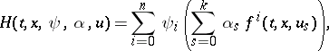
The Hamilton function for the problem (16)–(19), | The Hamilton function for the problem (16)–(19), | ||
| − | + | <table class="eq" style="width:100%;"> <tr><td valign="top" style="width:94%;text-align:center;"><img align="absmiddle" border="0" src="https://www.encyclopediaofmath.org/legacyimages/o/o068/o068490/o06849091.png" /></td> </tr></table> | |
| − | |||
| − | |||
| − | |||
| − | |||
| − | after excluding | + | after excluding <img align="absmiddle" border="0" src="https://www.encyclopediaofmath.org/legacyimages/o/o068/o068490/o06849092.png" /> and regrouping the terms, can be reduced to the form |
| − | and regrouping the terms, can be reduced to the form | ||
| − | + | <table class="eq" style="width:100%;"> <tr><td valign="top" style="width:94%;text-align:center;"><img align="absmiddle" border="0" src="https://www.encyclopediaofmath.org/legacyimages/o/o068/o068490/o06849093.png" /></td> <td valign="top" style="width:5%;text-align:right;">(20)</td></tr></table> | |
| − | |||
| − | |||
| − | + | <table class="eq" style="width:100%;"> <tr><td valign="top" style="width:94%;text-align:center;"><img align="absmiddle" border="0" src="https://www.encyclopediaofmath.org/legacyimages/o/o068/o068490/o06849094.png" /></td> </tr></table> | |
| − | = | ||
| − | |||
| − | |||
| − | |||
| − | + | <table class="eq" style="width:100%;"> <tr><td valign="top" style="width:94%;text-align:center;"><img align="absmiddle" border="0" src="https://www.encyclopediaofmath.org/legacyimages/o/o068/o068490/o06849095.png" /></td> </tr></table> | |
| − | = | ||
| − | |||
| − | |||
| − | Because the | + | Because the <img align="absmiddle" border="0" src="https://www.encyclopediaofmath.org/legacyimages/o/o068/o068490/o06849096.png" />, <img align="absmiddle" border="0" src="https://www.encyclopediaofmath.org/legacyimages/o/o068/o068490/o06849097.png" />, are equal to the maxima of <img align="absmiddle" border="0" src="https://www.encyclopediaofmath.org/legacyimages/o/o068/o068490/o06849098.png" /> with respect to <img align="absmiddle" border="0" src="https://www.encyclopediaofmath.org/legacyimages/o/o068/o068490/o06849099.png" /> on the set <img align="absmiddle" border="0" src="https://www.encyclopediaofmath.org/legacyimages/o/o068/o068490/o068490100.png" />, on the section <img align="absmiddle" border="0" src="https://www.encyclopediaofmath.org/legacyimages/o/o068/o068490/o068490101.png" /> of the optimal sliding regime with <img align="absmiddle" border="0" src="https://www.encyclopediaofmath.org/legacyimages/o/o068/o068490/o068490102.png" /> maxima the coefficients at the <img align="absmiddle" border="0" src="https://www.encyclopediaofmath.org/legacyimages/o/o068/o068490/o068490103.png" /> independent linear controls <img align="absmiddle" border="0" src="https://www.encyclopediaofmath.org/legacyimages/o/o068/o068490/o068490104.png" /> of the Hamilton function of the split problem (12)–(15) are equal to zero. An optimal sliding regime with a "slide" through <img align="absmiddle" border="0" src="https://www.encyclopediaofmath.org/legacyimages/o/o068/o068490/o068490105.png" /> maxima is an optimal singular regime with <img align="absmiddle" border="0" src="https://www.encyclopediaofmath.org/legacyimages/o/o068/o068490/o068490106.png" /> components for the split problem (16)–(19). The maximum possible value of <img align="absmiddle" border="0" src="https://www.encyclopediaofmath.org/legacyimages/o/o068/o068490/o068490107.png" /> advisable to take when researching sliding regimes is defined by the condition of convexity of the set of values of the right-hand side vector and the convexity from below of the greatest lower bound of the set of values of the integrand of the split system obtained when the control vector <img align="absmiddle" border="0" src="https://www.encyclopediaofmath.org/legacyimages/o/o068/o068490/o068490108.png" />, <img align="absmiddle" border="0" src="https://www.encyclopediaofmath.org/legacyimages/o/o068/o068490/o068490109.png" />, runs through the whole admissible domain of values. Thus, <img align="absmiddle" border="0" src="https://www.encyclopediaofmath.org/legacyimages/o/o068/o068490/o068490110.png" /> is an estimation from above for <img align="absmiddle" border="0" src="https://www.encyclopediaofmath.org/legacyimages/o/o068/o068490/o068490111.png" />. In the most general case, all optimal sliding regimes of the initial problem can be obtained as optimal singular controls of the split problem written out for <img align="absmiddle" border="0" src="https://www.encyclopediaofmath.org/legacyimages/o/o068/o068490/o068490112.png" />. In particular, in the above example, the split problem has been examined when <img align="absmiddle" border="0" src="https://www.encyclopediaofmath.org/legacyimages/o/o068/o068490/o068490113.png" />, insofar as the constraints contain only one equation; investigation into the split problem (8)–(11) has proved adequate for research into the optimal sliding regime of the initial problem (1)–(4). |
| − | |||
| − | are equal to the maxima of | ||
| − | with respect to | ||
| − | on the set | ||
| − | on the section | ||
| − | of the optimal sliding regime with | ||
| − | maxima the coefficients at the | ||
| − | independent linear controls | ||
| − | of the Hamilton function of the split problem (12)–(15) are equal to zero. An optimal sliding regime with a "slide" through | ||
| − | maxima is an optimal singular regime with | ||
| − | components for the split problem (16)–(19). The maximum possible value of | ||
| − | advisable to take when researching sliding regimes is defined by the condition of convexity of the set of values of the right-hand side vector and the convexity from below of the greatest lower bound of the set of values of the integrand of the split system obtained when the control vector | ||
| − | |||
| − | runs through the whole admissible domain of values. Thus, | ||
| − | is an estimation from above for | ||
| − | In the most general case, all optimal sliding regimes of the initial problem can be obtained as optimal singular controls of the split problem written out for | ||
| − | In particular, in the above example, the split problem has been examined when | ||
| − | insofar as the constraints contain only one equation; investigation into the split problem (8)–(11) has proved adequate for research into the optimal sliding regime of the initial problem (1)–(4). | ||
| − | If | + | If <img align="absmiddle" border="0" src="https://www.encyclopediaofmath.org/legacyimages/o/o068/o068490/o068490114.png" /> and controls <img align="absmiddle" border="0" src="https://www.encyclopediaofmath.org/legacyimages/o/o068/o068490/o068490115.png" /> are known which provide equal absolute maxima of the Hamilton function <img align="absmiddle" border="0" src="https://www.encyclopediaofmath.org/legacyimages/o/o068/o068490/o068490116.png" /> in the admissible domain <img align="absmiddle" border="0" src="https://www.encyclopediaofmath.org/legacyimages/o/o068/o068490/o068490117.png" />, then the analysis of the optimal sliding regime reduces to the investigation of an optimal singular regime with <img align="absmiddle" border="0" src="https://www.encyclopediaofmath.org/legacyimages/o/o068/o068490/o068490118.png" /> components. This investigation can be carried out by using necessary conditions of optimality of a singular control (see [[Optimal singular regime|Optimal singular regime]]). |
| − | and controls | ||
| − | are known which provide equal absolute maxima of the Hamilton function | ||
| − | in the admissible domain | ||
| − | then the analysis of the optimal sliding regime reduces to the investigation of an optimal singular regime with | ||
| − | components. This investigation can be carried out by using necessary conditions of optimality of a singular control (see [[Optimal singular regime|Optimal singular regime]]). | ||
Investigations have been carried out into optimal sliding regimes using sufficient conditions of optimality (see [[#References|[4]]]). | Investigations have been carried out into optimal sliding regimes using sufficient conditions of optimality (see [[#References|[4]]]). | ||
| Line 313: | Line 119: | ||
====References==== | ====References==== | ||
<table><TR><TD valign="top">[1]</TD> <TD valign="top"> R.V. Gamkrelidze, "Optimal sliding states" ''Soviet Math. Dokl.'' , '''3''' : 2 (1962) pp. 559–562 ''Dokl. Akad. Nauk SSSR'' , '''143''' : 6 (1962) pp. 1243–1245</TD></TR><TR><TD valign="top">[2]</TD> <TD valign="top"> L.S. Pontryagin, V.G. Boltayanskii, R.V. Gamkrelidze, E.F. Mishchenko, "The mathematical theory of optimal processes" , Wiley (1967) (Translated from Russian)</TD></TR><TR><TD valign="top">[3]</TD> <TD valign="top"> I.B. Vapnyarskii, "An existence theorem for optimal control in the Boltz problem, some of its applications and the necessary conditions for the optimality of moving and singular systems" ''USSR Comp. Math. Math. Phys.'' , '''7''' : 2 (1963) pp. 22–54 ''Zh. Vychisl. Mat. i Mat. Fiz.'' , '''7''' : 2 (1967) pp. 259–283</TD></TR><TR><TD valign="top">[4]</TD> <TD valign="top"> V.F. Krotov, "Methods for solving variational problems based on sufficient conditions for an absolute minimum II" ''Automat. Remote Control'' , '''24''' (1963) pp. 539–553 ''Avtomatik. i Telemekh.'' , '''24''' : 5 (1963) pp. 581–598</TD></TR></table> | <table><TR><TD valign="top">[1]</TD> <TD valign="top"> R.V. Gamkrelidze, "Optimal sliding states" ''Soviet Math. Dokl.'' , '''3''' : 2 (1962) pp. 559–562 ''Dokl. Akad. Nauk SSSR'' , '''143''' : 6 (1962) pp. 1243–1245</TD></TR><TR><TD valign="top">[2]</TD> <TD valign="top"> L.S. Pontryagin, V.G. Boltayanskii, R.V. Gamkrelidze, E.F. Mishchenko, "The mathematical theory of optimal processes" , Wiley (1967) (Translated from Russian)</TD></TR><TR><TD valign="top">[3]</TD> <TD valign="top"> I.B. Vapnyarskii, "An existence theorem for optimal control in the Boltz problem, some of its applications and the necessary conditions for the optimality of moving and singular systems" ''USSR Comp. Math. Math. Phys.'' , '''7''' : 2 (1963) pp. 22–54 ''Zh. Vychisl. Mat. i Mat. Fiz.'' , '''7''' : 2 (1967) pp. 259–283</TD></TR><TR><TD valign="top">[4]</TD> <TD valign="top"> V.F. Krotov, "Methods for solving variational problems based on sufficient conditions for an absolute minimum II" ''Automat. Remote Control'' , '''24''' (1963) pp. 539–553 ''Avtomatik. i Telemekh.'' , '''24''' : 5 (1963) pp. 581–598</TD></TR></table> | ||
| + | |||
| + | |||
====Comments==== | ====Comments==== | ||
Revision as of 14:52, 7 June 2020
A term used in the theory of optimal control to describe an optimal method of controlling a system when a minimizing sequence of control functions does not have a limit in the class of Lebesgue-measurable functions.
For example, suppose a minimum of the functional
 | (1) |
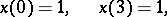
has to be found, given the constraints
 | (2) |
 | (3) |
 | (4) |
In order to obtain a minimum of the functional (1), it is desirable for every  to have as small a value as possible of
  and as large a value as possible of
  . The first requirement, with regard to the constraining condition (2), the boundary conditions (3) and the control constraint (4), is satisfied by the trajectory
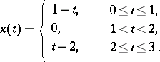 | (5) |
If the trajectory (5) could be created for a control which, for all  , has the boundary values
 | (6) |
the absolute minimum of the functional (1) would be obtained. However, the "ideal" trajectory (5) cannot be created for any control function  which satisfies (6), since, when
  ,
,  . Nevertheless, it is possible, using control functions
  which, when
  and
and  , realize ever more frequent switchings from 1 to
  and vice versa:
 | (7) |
 |
( ), to create a minimizing sequence of controls
  which satisfies (6) and a minimizing sequence of trajectories
  converging towards the "ideal" trajectory (5).
Each trajectory  differs from (5) only on the interval
  on which, instead of being a precise path along the
  -axis, it makes a "saw-toothed" path with
  identical "teeth" , positioned above the
  -axis. The "teeth of the saw" become ever finer when
  , such that
 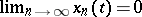 ,
,  . In this way, the minimizing sequence of trajectories
  converges towards (5), but the minimizing sequence of controls
  , which, when
  and
and  , realizes ever more frequent switchings from 1 to
  and vice versa, does not have a limit in the class of measurable (and even more so in the class of piecewise continuous) functions. This means that on the section
  an optimal sliding regime occurs.
Using heuristic reasoning, it is possible to describe the optimal sliding regime obtained in the following way: An optimal control at each point of the interval  "slides" , i.e. skips from the value
  to
to  and back, such that, for any interval of time, however small, the measure of the set of points
  in which
  is equal to the measure of the set of points
  in which
  , which, by virtue of equation (2), ensures a precise motion along the
  -axis. The description given above of the character of change of an optimal control on part of a sliding regime is non-rigorous, for it does not satisfy the ordinary definition of a function.
It is possible to give a rigorous definition of an optimal sliding regime if, along with the initial problem (1)–(4), an auxiliary "split" problem is introduced: To find a minimum of the functional
 | (8) |
given the constraints
 | (9) |
 | (10) |
 | (11) |
The split problem (8)–(11) differs from the initial one in that, instead of one control function  , two independent control functions
  and
and  are introduced; the integrand and the function on the right-hand side of equation (2) of the initial problem are replaced by a linear convex combination of corresponding functions, taken with different controls
  and
and  and with coefficients
  ,
,  , which are also considered as control functions.
Thus, in problem (8)–(11) there are four controls  ,
,  ,
,  ,
,  . Insofar as
  and
and  are related by the equality-type condition
 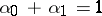 , it is possible to drop one of the controls
  or
or  by expressing it through the other. However, for the convenience of subsequent analysis, it is advisable to leave both controls in an explicit form.
Unlike the initial problem, an optimal control for the split problem (8)–(11) exists. On a section of the optimal sliding regime of the initial problem, the optimal control for the split problem takes the form
 |
 |
while on the sections of entry and exit:
 |
 |
 |
 |
 |
 |
On the section of an optimal sliding regime, the controls  and
and  , going linearly into the right-hand side, and the integrand accept values within the admissible domain. This means that the optimal sliding regime of the initial problem (1)–(4) is an optimal singular regime, or optimal singular control, for the auxiliary split problem (8)–(11).
The same results occur for optimal sliding regimes in general problems of optimal control. Suppose that a minimum of the functional
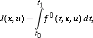 | (12) |
 |
has to be found, given the conditions
 | (13) |
 | (14) |
 | (15) |
The optimal sliding regime is characterized by the non-uniqueness of the maximum with respect to  of the Hamilton function
 |
where  are conjugate variables (see [2]). Under these conditions, on the section
  of the
  -st "slide"
  with the maxima
  , the initial problem splits and takes the form
 | (16) |
 | (17) |
 | (18) |
 | (19) |
The Hamilton function for the problem (16)–(19),
 |
after excluding  and regrouping the terms, can be reduced to the form
 | (20) |
 |
 |
Because the  ,
,  , are equal to the maxima of
  with respect to
  on the set
  , on the section
  of the optimal sliding regime with
  maxima the coefficients at the
  independent linear controls
  of the Hamilton function of the split problem (12)–(15) are equal to zero. An optimal sliding regime with a "slide" through
  maxima is an optimal singular regime with
  components for the split problem (16)–(19). The maximum possible value of
  advisable to take when researching sliding regimes is defined by the condition of convexity of the set of values of the right-hand side vector and the convexity from below of the greatest lower bound of the set of values of the integrand of the split system obtained when the control vector
  ,
,  , runs through the whole admissible domain of values. Thus,
  is an estimation from above for
  . In the most general case, all optimal sliding regimes of the initial problem can be obtained as optimal singular controls of the split problem written out for
  . In particular, in the above example, the split problem has been examined when
  , insofar as the constraints contain only one equation; investigation into the split problem (8)–(11) has proved adequate for research into the optimal sliding regime of the initial problem (1)–(4).
If  and controls
  are known which provide equal absolute maxima of the Hamilton function
  in the admissible domain
  , then the analysis of the optimal sliding regime reduces to the investigation of an optimal singular regime with
  components. This investigation can be carried out by using necessary conditions of optimality of a singular control (see Optimal singular regime).
Investigations have been carried out into optimal sliding regimes using sufficient conditions of optimality (see [4]).
References
| [1] | R.V. Gamkrelidze, "Optimal sliding states" Soviet Math. Dokl. , 3 : 2 (1962) pp. 559–562 Dokl. Akad. Nauk SSSR , 143 : 6 (1962) pp. 1243–1245 |
| [2] | L.S. Pontryagin, V.G. Boltayanskii, R.V. Gamkrelidze, E.F. Mishchenko, "The mathematical theory of optimal processes" , Wiley (1967) (Translated from Russian) |
| [3] | I.B. Vapnyarskii, "An existence theorem for optimal control in the Boltz problem, some of its applications and the necessary conditions for the optimality of moving and singular systems" USSR Comp. Math. Math. Phys. , 7 : 2 (1963) pp. 22–54 Zh. Vychisl. Mat. i Mat. Fiz. , 7 : 2 (1967) pp. 259–283 |
| [4] | V.F. Krotov, "Methods for solving variational problems based on sufficient conditions for an absolute minimum II" Automat. Remote Control , 24 (1963) pp. 539–553 Avtomatik. i Telemekh. , 24 : 5 (1963) pp. 581–598 |
Comments
A sliding control is also called a chattering control, see [a1].
For more references see also Optimal singular regime.
References
| [a1] | L. Markus, "Foundations of optimal control theory" , Wiley (1967) |
Optimal sliding regime. Encyclopedia of Mathematics. URL: http://encyclopediaofmath.org/index.php?title=Optimal_sliding_regime&oldid=49342