Difference between revisions of "Neyman method of confidence intervals"
Ulf Rehmann (talk | contribs) m (tex encoded by computer) |
Ulf Rehmann (talk | contribs) m (Undo revision 47969 by Ulf Rehmann (talk)) Tag: Undo |
||
| Line 1: | Line 1: | ||
| − | < | + | One of the methods of [[Confidence estimation|confidence estimation]], which makes it possible to obtain interval estimators (cf. [[Interval estimator|Interval estimator]]) for unknown parameters of probability laws from results of observations. It was proposed and developed by J. Neyman (see [[#References|[1]]], [[#References|[2]]]). The essence of the method consists in the following. Let <img align="absmiddle" border="0" src="https://www.encyclopediaofmath.org/legacyimages/n/n066/n066590/n0665901.png" /> be random variables whose joint distribution function <img align="absmiddle" border="0" src="https://www.encyclopediaofmath.org/legacyimages/n/n066/n066590/n0665902.png" /> depends on a parameter <img align="absmiddle" border="0" src="https://www.encyclopediaofmath.org/legacyimages/n/n066/n066590/n0665903.png" />, <img align="absmiddle" border="0" src="https://www.encyclopediaofmath.org/legacyimages/n/n066/n066590/n0665904.png" />. Suppose, next, that as point estimator of the parameter <img align="absmiddle" border="0" src="https://www.encyclopediaofmath.org/legacyimages/n/n066/n066590/n0665905.png" /> a statistic <img align="absmiddle" border="0" src="https://www.encyclopediaofmath.org/legacyimages/n/n066/n066590/n0665906.png" /> is used with distribution function <img align="absmiddle" border="0" src="https://www.encyclopediaofmath.org/legacyimages/n/n066/n066590/n0665907.png" />, <img align="absmiddle" border="0" src="https://www.encyclopediaofmath.org/legacyimages/n/n066/n066590/n0665908.png" />. Then for any number <img align="absmiddle" border="0" src="https://www.encyclopediaofmath.org/legacyimages/n/n066/n066590/n0665909.png" /> in the interval <img align="absmiddle" border="0" src="https://www.encyclopediaofmath.org/legacyimages/n/n066/n066590/n06659010.png" /> one can define a system of two equations in <img align="absmiddle" border="0" src="https://www.encyclopediaofmath.org/legacyimages/n/n066/n066590/n06659011.png" />: |
| − | n0665901.png | ||
| − | |||
| − | |||
| − | |||
| − | |||
| − | |||
| − | |||
| − | + | <table class="eq" style="width:100%;"> <tr><td valign="top" style="width:94%;text-align:center;"><img align="absmiddle" border="0" src="https://www.encyclopediaofmath.org/legacyimages/n/n066/n066590/n06659012.png" /></td> <td valign="top" style="width:5%;text-align:right;">(*)</td></tr></table> | |
| − | |||
| − | + | Under certain regularity conditions on <img align="absmiddle" border="0" src="https://www.encyclopediaofmath.org/legacyimages/n/n066/n066590/n06659013.png" />, which in almost-all cases of practical interest are satisfied, the system (*) has a unique solution | |
| − | |||
| − | |||
| − | |||
| − | |||
| − | |||
| − | |||
| − | |||
| − | |||
| − | |||
| − | |||
| − | + | <table class="eq" style="width:100%;"> <tr><td valign="top" style="width:94%;text-align:center;"><img align="absmiddle" border="0" src="https://www.encyclopediaofmath.org/legacyimages/n/n066/n066590/n06659014.png" /></td> </tr></table> | |
| − | |||
| − | |||
| − | |||
| − | |||
| − | |||
| − | |||
| − | |||
| − | |||
| − | |||
| − | |||
| − | |||
| − | |||
| − | |||
such that | such that | ||
| − | + | <table class="eq" style="width:100%;"> <tr><td valign="top" style="width:94%;text-align:center;"><img align="absmiddle" border="0" src="https://www.encyclopediaofmath.org/legacyimages/n/n066/n066590/n06659015.png" /></td> </tr></table> | |
| − | |||
| − | |||
| − | |||
| − | The set | + | The set <img align="absmiddle" border="0" src="https://www.encyclopediaofmath.org/legacyimages/n/n066/n066590/n06659016.png" /> is called the confidence interval (confidence estimator) for the unknown parameter <img align="absmiddle" border="0" src="https://www.encyclopediaofmath.org/legacyimages/n/n066/n066590/n06659017.png" /> with confidence probability <img align="absmiddle" border="0" src="https://www.encyclopediaofmath.org/legacyimages/n/n066/n066590/n06659018.png" />. The statistics <img align="absmiddle" border="0" src="https://www.encyclopediaofmath.org/legacyimages/n/n066/n066590/n06659019.png" /> and <img align="absmiddle" border="0" src="https://www.encyclopediaofmath.org/legacyimages/n/n066/n066590/n06659020.png" /> are called the lower and upper confidence bounds corresponding to the chosen confidence coefficient <img align="absmiddle" border="0" src="https://www.encyclopediaofmath.org/legacyimages/n/n066/n066590/n06659021.png" />. In turn, the number |
| − | is called the confidence interval (confidence estimator) for the unknown parameter | ||
| − | with confidence probability | ||
| − | The statistics | ||
| − | and | ||
| − | are called the lower and upper confidence bounds corresponding to the chosen confidence coefficient | ||
| − | In turn, the number | ||
| − | + | <table class="eq" style="width:100%;"> <tr><td valign="top" style="width:94%;text-align:center;"><img align="absmiddle" border="0" src="https://www.encyclopediaofmath.org/legacyimages/n/n066/n066590/n06659022.png" /></td> </tr></table> | |
| − | |||
| − | |||
| − | |||
| − | is called the confidence coefficient of the confidence interval | + | is called the confidence coefficient of the confidence interval <img align="absmiddle" border="0" src="https://www.encyclopediaofmath.org/legacyimages/n/n066/n066590/n06659023.png" />. Thus, Neyman's method of confidence intervals leads to interval estimators with confidence coefficient <img align="absmiddle" border="0" src="https://www.encyclopediaofmath.org/legacyimages/n/n066/n066590/n06659024.png" />. |
| − | Thus, Neyman's method of confidence intervals leads to interval estimators with confidence coefficient | ||
| − | Example 1. Suppose that independent random variables | + | Example 1. Suppose that independent random variables <img align="absmiddle" border="0" src="https://www.encyclopediaofmath.org/legacyimages/n/n066/n066590/n06659025.png" /> are subject to one and the same normal law <img align="absmiddle" border="0" src="https://www.encyclopediaofmath.org/legacyimages/n/n066/n066590/n06659026.png" /> whose mathematical expectation <img align="absmiddle" border="0" src="https://www.encyclopediaofmath.org/legacyimages/n/n066/n066590/n06659027.png" /> is not known (cf. [[Normal distribution|Normal distribution]]). Then the best estimator for <img align="absmiddle" border="0" src="https://www.encyclopediaofmath.org/legacyimages/n/n066/n066590/n06659028.png" /> is the [[Sufficient statistic|sufficient statistic]] <img align="absmiddle" border="0" src="https://www.encyclopediaofmath.org/legacyimages/n/n066/n066590/n06659029.png" />, which is distributed according to the normal law <img align="absmiddle" border="0" src="https://www.encyclopediaofmath.org/legacyimages/n/n066/n066590/n06659030.png" />. Fixing <img align="absmiddle" border="0" src="https://www.encyclopediaofmath.org/legacyimages/n/n066/n066590/n06659031.png" /> in <img align="absmiddle" border="0" src="https://www.encyclopediaofmath.org/legacyimages/n/n066/n066590/n06659032.png" /> and solving the equations |
| − | are subject to one and the same normal law | ||
| − | whose mathematical expectation | ||
| − | is not known (cf. [[Normal distribution|Normal distribution]]). Then the best estimator for | ||
| − | is the [[Sufficient statistic|sufficient statistic]] | ||
| − | which is distributed according to the normal law | ||
| − | Fixing | ||
| − | in | ||
| − | and solving the equations | ||
| − | + | <table class="eq" style="width:100%;"> <tr><td valign="top" style="width:94%;text-align:center;"><img align="absmiddle" border="0" src="https://www.encyclopediaofmath.org/legacyimages/n/n066/n066590/n06659033.png" /></td> </tr></table> | |
| − | |||
| − | |||
| − | |||
one finds the lower and upper confidence bounds | one finds the lower and upper confidence bounds | ||
| − | + | <table class="eq" style="width:100%;"> <tr><td valign="top" style="width:94%;text-align:center;"><img align="absmiddle" border="0" src="https://www.encyclopediaofmath.org/legacyimages/n/n066/n066590/n06659034.png" /></td> </tr></table> | |
| − | |||
| − | |||
| − | |||
| − | |||
| − | |||
| − | |||
| − | |||
| − | corresponding to the chosen confidence coefficient | + | corresponding to the chosen confidence coefficient <img align="absmiddle" border="0" src="https://www.encyclopediaofmath.org/legacyimages/n/n066/n066590/n06659035.png" />. Since |
| − | Since | ||
| − | + | <table class="eq" style="width:100%;"> <tr><td valign="top" style="width:94%;text-align:center;"><img align="absmiddle" border="0" src="https://www.encyclopediaofmath.org/legacyimages/n/n066/n066590/n06659036.png" /></td> </tr></table> | |
| − | |||
| − | |||
| − | |||
| − | the confidence interval for the unknown mathematical expectation | + | the confidence interval for the unknown mathematical expectation <img align="absmiddle" border="0" src="https://www.encyclopediaofmath.org/legacyimages/n/n066/n066590/n06659037.png" /> of the normal law <img align="absmiddle" border="0" src="https://www.encyclopediaofmath.org/legacyimages/n/n066/n066590/n06659038.png" /> has the form |
| − | of the normal law | ||
| − | has the form | ||
| − | + | <table class="eq" style="width:100%;"> <tr><td valign="top" style="width:94%;text-align:center;"><img align="absmiddle" border="0" src="https://www.encyclopediaofmath.org/legacyimages/n/n066/n066590/n06659039.png" /></td> </tr></table> | |
| − | |||
| − | |||
| − | |||
| − | |||
| − | |||
| − | |||
| − | |||
| − | and its confidence coefficient is precisely | + | and its confidence coefficient is precisely <img align="absmiddle" border="0" src="https://www.encyclopediaofmath.org/legacyimages/n/n066/n066590/n06659040.png" />. |
| − | Example 2. Let | + | Example 2. Let <img align="absmiddle" border="0" src="https://www.encyclopediaofmath.org/legacyimages/n/n066/n066590/n06659041.png" /> be a random variable subject to the binomial law with parameters <img align="absmiddle" border="0" src="https://www.encyclopediaofmath.org/legacyimages/n/n066/n066590/n06659042.png" /> and <img align="absmiddle" border="0" src="https://www.encyclopediaofmath.org/legacyimages/n/n066/n066590/n06659043.png" /> (cf. [[Binomial distribution|Binomial distribution]]), that is, for any integer <img align="absmiddle" border="0" src="https://www.encyclopediaofmath.org/legacyimages/n/n066/n066590/n06659044.png" />, |
| − | be a random variable subject to the binomial law with parameters | ||
| − | and | ||
| − | cf. [[Binomial distribution|Binomial distribution]]), that is, for any integer | ||
| − | + | <table class="eq" style="width:100%;"> <tr><td valign="top" style="width:94%;text-align:center;"><img align="absmiddle" border="0" src="https://www.encyclopediaofmath.org/legacyimages/n/n066/n066590/n06659045.png" /></td> </tr></table> | |
| − | |||
| − | |||
| − | |||
| − | n | ||
| − | |||
| − | |||
| − | |||
| − | |||
| − | |||
| − | + | <table class="eq" style="width:100%;"> <tr><td valign="top" style="width:94%;text-align:center;"><img align="absmiddle" border="0" src="https://www.encyclopediaofmath.org/legacyimages/n/n066/n066590/n06659046.png" /></td> </tr></table> | |
| − | = | ||
| − | |||
| − | |||
where | where | ||
| − | + | <table class="eq" style="width:100%;"> <tr><td valign="top" style="width:94%;text-align:center;"><img align="absmiddle" border="0" src="https://www.encyclopediaofmath.org/legacyimages/n/n066/n066590/n06659047.png" /></td> </tr></table> | |
| − | |||
| − | |||
| − | |||
| − | |||
| − | |||
| − | |||
| − | |||
| − | is the [[Incomplete beta-function|incomplete beta-function]] ( | + | is the [[Incomplete beta-function|incomplete beta-function]] (<img align="absmiddle" border="0" src="https://www.encyclopediaofmath.org/legacyimages/n/n066/n066590/n06659048.png" />, <img align="absmiddle" border="0" src="https://www.encyclopediaofmath.org/legacyimages/n/n066/n066590/n06659049.png" />, <img align="absmiddle" border="0" src="https://www.encyclopediaofmath.org/legacyimages/n/n066/n066590/n06659050.png" />). If the "success" parameter <img align="absmiddle" border="0" src="https://www.encyclopediaofmath.org/legacyimages/n/n066/n066590/n06659051.png" /> is not known, then to determine the confidence bounds one has to solve, in accordance with Neyman's method of confidence intervals, the equations |
| − | |||
| − | |||
| − | If the "success" parameter | ||
| − | is not known, then to determine the confidence bounds one has to solve, in accordance with Neyman's method of confidence intervals, the equations | ||
| − | + | <table class="eq" style="width:100%;"> <tr><td valign="top" style="width:94%;text-align:center;"><img align="absmiddle" border="0" src="https://www.encyclopediaofmath.org/legacyimages/n/n066/n066590/n06659052.png" /></td> </tr></table> | |
| − | |||
| − | |||
| − | where | + | where <img align="absmiddle" border="0" src="https://www.encyclopediaofmath.org/legacyimages/n/n066/n066590/n06659053.png" />. From tables of mathematical statistics the roots <img align="absmiddle" border="0" src="https://www.encyclopediaofmath.org/legacyimages/n/n066/n066590/n06659054.png" /> and <img align="absmiddle" border="0" src="https://www.encyclopediaofmath.org/legacyimages/n/n066/n066590/n06659055.png" /> of these equations are determined, which are the upper and lower confidence bounds, respectively, with confidence coefficient <img align="absmiddle" border="0" src="https://www.encyclopediaofmath.org/legacyimages/n/n066/n066590/n06659056.png" />. The coefficient of the resulting confidence interval <img align="absmiddle" border="0" src="https://www.encyclopediaofmath.org/legacyimages/n/n066/n066590/n06659057.png" /> is precisely <img align="absmiddle" border="0" src="https://www.encyclopediaofmath.org/legacyimages/n/n066/n066590/n06659058.png" />. Obviously, if an experiment gives <img align="absmiddle" border="0" src="https://www.encyclopediaofmath.org/legacyimages/n/n066/n066590/n06659059.png" />, then <img align="absmiddle" border="0" src="https://www.encyclopediaofmath.org/legacyimages/n/n066/n066590/n06659060.png" />, and if <img align="absmiddle" border="0" src="https://www.encyclopediaofmath.org/legacyimages/n/n066/n066590/n06659061.png" />, then <img align="absmiddle" border="0" src="https://www.encyclopediaofmath.org/legacyimages/n/n066/n066590/n06659062.png" />. |
| − | From tables of mathematical statistics the roots | ||
| − | and | ||
| − | of these equations are determined, which are the upper and lower confidence bounds, respectively, with confidence coefficient | ||
| − | The coefficient of the resulting confidence interval | ||
| − | is precisely | ||
| − | Obviously, if an experiment gives | ||
| − | then | ||
| − | and if | ||
| − | then | ||
| − | Neyman's method of confidence intervals differs substantially from the Bayesian method (cf. [[Bayesian approach|Bayesian approach]]) and the method based on Fisher's fiducial approach (cf. [[Fiducial distribution|Fiducial distribution]]). In it the unknown parameter | + | Neyman's method of confidence intervals differs substantially from the Bayesian method (cf. [[Bayesian approach|Bayesian approach]]) and the method based on Fisher's fiducial approach (cf. [[Fiducial distribution|Fiducial distribution]]). In it the unknown parameter <img align="absmiddle" border="0" src="https://www.encyclopediaofmath.org/legacyimages/n/n066/n066590/n06659063.png" /> of the distribution function <img align="absmiddle" border="0" src="https://www.encyclopediaofmath.org/legacyimages/n/n066/n066590/n06659064.png" /> is treated as a constant quantity, and the confidence interval <img align="absmiddle" border="0" src="https://www.encyclopediaofmath.org/legacyimages/n/n066/n066590/n06659065.png" /> is constructed from an experiment in the course of which the value of the statistic <img align="absmiddle" border="0" src="https://www.encyclopediaofmath.org/legacyimages/n/n066/n066590/n06659066.png" /> is calculated. Consequently, according to Neyman's method of confidence intervals, the probability for <img align="absmiddle" border="0" src="https://www.encyclopediaofmath.org/legacyimages/n/n066/n066590/n06659067.png" /> to hold is the [[A priori probability|a priori probability]] for the fact that the confidence interval <img align="absmiddle" border="0" src="https://www.encyclopediaofmath.org/legacyimages/n/n066/n066590/n06659068.png" /> "covers" the unknown true value of the parameter <img align="absmiddle" border="0" src="https://www.encyclopediaofmath.org/legacyimages/n/n066/n066590/n06659069.png" />. In fact, Neyman's confidence method remains valid if <img align="absmiddle" border="0" src="https://www.encyclopediaofmath.org/legacyimages/n/n066/n066590/n06659070.png" /> is a random variable, because in the method the interval estimator is constructed from carrying out an experiment and consequently does not depend on the [[A priori distribution|a priori distribution]] of the parameter. Neyman's method differs advantageously from the Bayesian and the fiducial approach by being independent of a priori information about the parameter <img align="absmiddle" border="0" src="https://www.encyclopediaofmath.org/legacyimages/n/n066/n066590/n06659071.png" /> and so, in contrast to Fisher's method, is logically sound. In general, Neyman's method leads to a whole system of confidence intervals for the unknown parameter, and in this context arises the problem of constructing an optimal interval estimator having, for example, the properties of being unbiased, accurate or similar, which can be solved within the framework of the theory of statistical hypothesis testing. |
| − | of the distribution function | ||
| − | is treated as a constant quantity, and the confidence interval | ||
| − | is constructed from an experiment in the course of which the value of the statistic | ||
| − | is calculated. Consequently, according to Neyman's method of confidence intervals, the probability for | ||
| − | to hold is the [[A priori probability|a priori probability]] for the fact that the confidence interval | ||
| − | covers" the unknown true value of the parameter | ||
| − | In fact, Neyman's confidence method remains valid if | ||
| − | is a random variable, because in the method the interval estimator is constructed from carrying out an experiment and consequently does not depend on the [[A priori distribution|a priori distribution]] of the parameter. Neyman's method differs advantageously from the Bayesian and the fiducial approach by being independent of a priori information about the parameter | ||
| − | and so, in contrast to Fisher's method, is logically sound. In general, Neyman's method leads to a whole system of confidence intervals for the unknown parameter, and in this context arises the problem of constructing an optimal interval estimator having, for example, the properties of being unbiased, accurate or similar, which can be solved within the framework of the theory of statistical hypothesis testing. | ||
====References==== | ====References==== | ||
<table><TR><TD valign="top">[1]</TD> <TD valign="top"> J. Neyman, "On the problem of confidence intervals" ''Ann. Math. Stat.'' , '''6''' (1935) pp. 111–116</TD></TR><TR><TD valign="top">[2]</TD> <TD valign="top"> J. Neyman, "Outline of a theory of statistical estimation based on the classical theory of probability" ''Philos. Trans. Roy. Soc. London. Ser. A.'' , '''236''' (1937) pp. 333–380</TD></TR><TR><TD valign="top">[3]</TD> <TD valign="top"> L.N. Bol'shev, N.V. Smirnov, "Tables of mathematical statistics" , ''Libr. math. tables'' , '''46''' , Nauka (1983) (In Russian) (Processed by L.S. Bark and E.S. Kedrova)</TD></TR><TR><TD valign="top">[4]</TD> <TD valign="top"> L.N. Bol'shev, "On the construction of confidence limits" ''Theor. Probab. Appl.'' , '''10''' (1965) pp. 173–177 ''Teor. Veroyatnost. i Primenen.'' , '''10''' : 1 (1965) pp. 187–192</TD></TR><TR><TD valign="top">[5]</TD> <TD valign="top"> E.L. Lehmann, "Testing statistical hypotheses" , Wiley (1986)</TD></TR></table> | <table><TR><TD valign="top">[1]</TD> <TD valign="top"> J. Neyman, "On the problem of confidence intervals" ''Ann. Math. Stat.'' , '''6''' (1935) pp. 111–116</TD></TR><TR><TD valign="top">[2]</TD> <TD valign="top"> J. Neyman, "Outline of a theory of statistical estimation based on the classical theory of probability" ''Philos. Trans. Roy. Soc. London. Ser. A.'' , '''236''' (1937) pp. 333–380</TD></TR><TR><TD valign="top">[3]</TD> <TD valign="top"> L.N. Bol'shev, N.V. Smirnov, "Tables of mathematical statistics" , ''Libr. math. tables'' , '''46''' , Nauka (1983) (In Russian) (Processed by L.S. Bark and E.S. Kedrova)</TD></TR><TR><TD valign="top">[4]</TD> <TD valign="top"> L.N. Bol'shev, "On the construction of confidence limits" ''Theor. Probab. Appl.'' , '''10''' (1965) pp. 173–177 ''Teor. Veroyatnost. i Primenen.'' , '''10''' : 1 (1965) pp. 187–192</TD></TR><TR><TD valign="top">[5]</TD> <TD valign="top"> E.L. Lehmann, "Testing statistical hypotheses" , Wiley (1986)</TD></TR></table> | ||
Revision as of 14:52, 7 June 2020
One of the methods of confidence estimation, which makes it possible to obtain interval estimators (cf. Interval estimator) for unknown parameters of probability laws from results of observations. It was proposed and developed by J. Neyman (see [1], [2]). The essence of the method consists in the following. Let  be random variables whose joint distribution function
  depends on a parameter
  ,
,  . Suppose, next, that as point estimator of the parameter
  a statistic
  is used with distribution function
  ,
,  . Then for any number
  in the interval
  one can define a system of two equations in
  :
:
 | (*) |
Under certain regularity conditions on  , which in almost-all cases of practical interest are satisfied, the system (*) has a unique solution
 |
such that
 |
The set  is called the confidence interval (confidence estimator) for the unknown parameter
  with confidence probability
  . The statistics
  and
and  are called the lower and upper confidence bounds corresponding to the chosen confidence coefficient
  . In turn, the number
 |
is called the confidence coefficient of the confidence interval  . Thus, Neyman's method of confidence intervals leads to interval estimators with confidence coefficient
  .
.
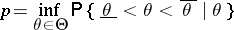
Example 1. Suppose that independent random variables  are subject to one and the same normal law
  whose mathematical expectation
  is not known (cf. Normal distribution). Then the best estimator for
  is the sufficient statistic
 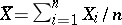 , which is distributed according to the normal law
 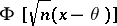 . Fixing
  in
in  and solving the equations
 |
one finds the lower and upper confidence bounds
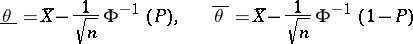 |
corresponding to the chosen confidence coefficient  . Since
 |
the confidence interval for the unknown mathematical expectation  of the normal law
  has the form
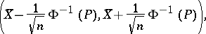 |
and its confidence coefficient is precisely  .
.
Example 2. Let  be a random variable subject to the binomial law with parameters
  and
and  (cf. Binomial distribution), that is, for any integer
  ,
,
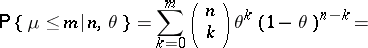 |
 |
where
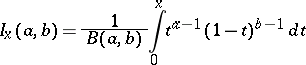 |
is the incomplete beta-function ( ,
,  ,
,  ). If the "success" parameter
  is not known, then to determine the confidence bounds one has to solve, in accordance with Neyman's method of confidence intervals, the equations
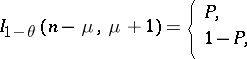 |
where  . From tables of mathematical statistics the roots
  and
and  of these equations are determined, which are the upper and lower confidence bounds, respectively, with confidence coefficient
  . The coefficient of the resulting confidence interval
  is precisely
  . Obviously, if an experiment gives
  , then
  , and if
  , then
  .
.
Neyman's method of confidence intervals differs substantially from the Bayesian method (cf. Bayesian approach) and the method based on Fisher's fiducial approach (cf. Fiducial distribution). In it the unknown parameter  of the distribution function
  is treated as a constant quantity, and the confidence interval
  is constructed from an experiment in the course of which the value of the statistic
  is calculated. Consequently, according to Neyman's method of confidence intervals, the probability for
  to hold is the a priori probability for the fact that the confidence interval
  "covers" the unknown true value of the parameter
  . In fact, Neyman's confidence method remains valid if
  is a random variable, because in the method the interval estimator is constructed from carrying out an experiment and consequently does not depend on the a priori distribution of the parameter. Neyman's method differs advantageously from the Bayesian and the fiducial approach by being independent of a priori information about the parameter
  and so, in contrast to Fisher's method, is logically sound. In general, Neyman's method leads to a whole system of confidence intervals for the unknown parameter, and in this context arises the problem of constructing an optimal interval estimator having, for example, the properties of being unbiased, accurate or similar, which can be solved within the framework of the theory of statistical hypothesis testing.
References
| [1] | J. Neyman, "On the problem of confidence intervals" Ann. Math. Stat. , 6 (1935) pp. 111–116 |
| [2] | J. Neyman, "Outline of a theory of statistical estimation based on the classical theory of probability" Philos. Trans. Roy. Soc. London. Ser. A. , 236 (1937) pp. 333–380 |
| [3] | L.N. Bol'shev, N.V. Smirnov, "Tables of mathematical statistics" , Libr. math. tables , 46 , Nauka (1983) (In Russian) (Processed by L.S. Bark and E.S. Kedrova) |
| [4] | L.N. Bol'shev, "On the construction of confidence limits" Theor. Probab. Appl. , 10 (1965) pp. 173–177 Teor. Veroyatnost. i Primenen. , 10 : 1 (1965) pp. 187–192 |
| [5] | E.L. Lehmann, "Testing statistical hypotheses" , Wiley (1986) |
Neyman method of confidence intervals. Encyclopedia of Mathematics. URL: http://encyclopediaofmath.org/index.php?title=Neyman_method_of_confidence_intervals&oldid=49328