Linear boundary value problem, numerical methods
Methods that make it possible to obtain a solution of a linear boundary value problem in the form of a table of approximate values of it at points of a grid, without using preliminary information about the expected form of the solution. In the theory of these methods it is typical to assume that the solution of the original problem exists and has sufficiently many derivatives. Because of the absence of other assumptions numerical methods differ in their universality.
Fundamental to numerical methods for solving a linear boundary value problem is the replacement of the original system of equations by its grid approximation. In the case of integro-differential equations such an approximation is usually constructed by means of difference schemes and quadrature formulas. The following problems arise:
1) How quickly does the exact solution of the grid problem converge to the solution of the original problem under refinement of the grid?
2) How sensitive is the solution of the grid problem to changes in the initial data?
3) How to find, at least approximately, the solution of the grid problem?
In the solution of the first and second problems the following apparatus is used. Suppose that in a closed domain  one is given the equation
 | (1) |
and on its boundary  , consisting of components
  , one is given the boundary conditions
 | (2) |
Here the given continuous functions  and
and  belong to some normed linear spaces
  and
and  , respectively, and the linear operators
  and
and  transform a certain linear subset
  of the normed linear space
  of functions that are continuous in
  into
into  and
and  , respectively.
Suppose that for an approximation of equation (1) one has chosen grids  and
and  that depend on a positive parameter
  , normed linear spaces
  and
and  of functions
  and
and  defined at the points of the grids
  and
and  , respectively, and also a linear operator
  that transforms
  into
into  . For an approximation of the boundary condition (2) one chooses a grid
  , a normed linear space
  of functions
  defined at the points of the grid
  , and a linear operator
  that transforms
  into
into  . Furthermore, one chooses linear operators
  and
and  that transform
  and
and  into
into  and
and  , respectively. As a result one obtains a grid approximation
 | (3) |
 | (4) |
of the original problem (1), (2). Let  ,
,  ,
,  denote the traces (restrictions) of the functions
  ,
,  ,
,  belonging to
  ,
,  ,
,  on the grids
  ,
,  ,
,  , respectively. It makes sense to carry out an investigation of the convergence of the grid approximations
  to the solution
  of the original problem as
  only in grid norms compatible with the norms in
  ,
,  ,
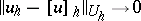
,  , that is, on the condition that for any functions
  ,
,  ,
,  the limit relations
 |
 |
hold. If  ,
,  ,
,  , then the quantity
 |
 |
is called the error of approximation of the problem (1), (2) by the problem (3), (4). If  is the solution of the problem (1), (2), then the quantity
 |
is called the error of approximation on this solution. One says that the problem (3), (4) approximates the problem (1), (2) (or approximates it on the solution  ) if
) if  (or
(or  ) as
) as  . The order of smallness of
  (or
(or  ) is called the order of approximation (or the order of approximation on the solution
  ).
).
Suppose, for example, that the heat equation is approximated. In the quadrant  (
( ) equation (1) is to be solved, where
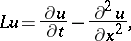 |
under the initial condition  on the half-line
  (
( ) and the boundary condition
  on the half-line
  (
( ), where
  ,
,  , and
, and  . For
. For  one chooses the space of continuous functions
  with the norm
 |
and for  and
and  one chooses the spaces of continuous functions
  and
and  with the norms
 |
respectively. One may assume that  coincides with
  , and for
  one chooses the subset of functions
  that have continuous partial derivatives
  ,
,  ,
,  in
in  . Let
. Let  be the set of points
  ,
,  ;
;  where the steps of the grid are connected by a functional dependence of the form
  such that
  as
as  . The set
  will consist of the points
  ,
,  ;
;  . For
. For  and
and  one chooses the spaces of grid functions
  and
and  with the compatible norms
 |
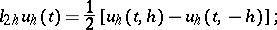
The operator  can be defined by the relation
 |
 |
 |
let
 |
For an approximation of the initial condition one chooses the grid  consisting of the points
  ,
,  the space
  of grid functions
  with the compatible norm
 |
and
 |
For an approximation of the boundary condition one chooses the grid  consisting of the points
  ,
,  ; the space
  of grid functions
  with the compatible norm
 |
the operator  defined by
 |
and the operator  . Then
 |
and  as
as  . If for
  one takes the more restricted set of functions
  having, apart from those mentioned above, bounded partial derivatives
  and
and  in
in  , then for
  one obtains an approximation of order two.
The grid problem
 | (3prm) |
 | (4prm) |
is said to be well-posed if for sufficiently small  the following conditions are satisfied: The problem is solvable for any given functions
  ,
,  and there is a function
  , independent of
  , that tends to zero together with
  and is such that
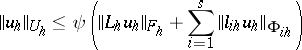 | (5) |
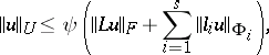
for any function  . The solution of a well-posed grid problem depends continuously on the given functions, uniformly with respect to
  . The fact that a grid problem is well-posed is a necessary condition for small sensitivity of its solution to rounding in the course of computation. If
  is the solution of (1), (2) and if the problem (3prm), (4prm) is well-posed, then
 | (6) |
Moreover, if the problem (3), (4) approximates the problem (1), (2) on the solution  , then
 |
as  . If the condition for compatibility of the norms, the condition
  and condition (5) are satisfied, then by putting
  and by a limit transition in (5) as
  , one obtains the inequality
 | (7) |
which is true for any function  . Thus, to investigate whether boundary value problems of the form (1), (2) are well-posed one can proceed as follows: first obtain an estimate (5), and from it estimate (7). By means of estimates of the type (5) one can often prove the existence of a solution
  of the problem (1), (2) as the limit of the grid approximations
  as
as  .
.
For a complete solution of the problem of finding an approximate solution of the problem (1), (2) it is necessary to construct an exact or approximate method for finding a solution of the approximation (3), (4) that has the property of stability to rounding. To investigate stability it is useful to use the concept of closure of a computational algorithm. In the given example it is advisable to solve the equation by the double-sweep method with respect to the variable  .
.
The estimate (6) of the error of the grid method has the disadvantage that in the expression of the function  derivatives of the exact solution
  usually occur. In some cases one can estimate these derivatives a priori (that is, before giving a solution of the problem), but such estimates usually turn out to be coarse. There are somewhat more accurate estimates in which the derivatives are replaced by difference quotients of the approximate solution
  . A practical estimation of the error of grid methods is mainly carried out by means of repeated solutions of the problem (3), (4) with various
  and subsequent isolation of the main part of the error of the form
  , where
  is the known order of smallness of the error. Thus, if one has the asymptotic relation
 |
then
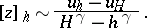 |
One can sometimes obtain equations for  that contain derivatives of the exact solution
  . Then one can solve them numerically on a coarser grid after solving the original problem, obtain the main error term and add it to the approximate solution
  , thereby refining it.
In some cases, using a special choice of the coordinate functions in variation or projection methods for solving the problem (1), (2) one obtains equations of the form (3), (4) that ensure convergence not only to the classical but also to the generalized solution. This method of constructing approximations, sometimes called the finite-element method, allows great freedom in the choice of the grid. The possibility of appropriately arranging the nodes makes it possible to attain the required accuracy with fewer nodes of the grid.
References
| [1] | I. [I. Babushka] Babuška, M. Práger, E. Vitásek, "Numerical processes in differential equations" , SNTL (1966) |
| [2] | N.S. Bakhvalov, "Summary of the course "Foundations of computational mathematics" " , 4 , Moscow (1968) (In Russian) |
| [3] | N.S. Bakhvalov, "Numerical methods: analysis, algebra, ordinary differential equations" , MIR (1977) (Translated from Russian) |
| [4] | R.S. Varga, "Functional analysis and approximation theory in numerical analysis" , Reg. Conf. Ser. Appl. Math. , 3 , SIAM (1971) |
| [5] | M.K. Gavurin, "Lectures on computing methods" , Moscow (1971) (In Russian) |
| [6] | S.K. Godunov, V.S. Ryaben'kii, "The theory of difference schemes" , North-Holland (1964) (Translated from Russian) |
| [7] | E.G. D'yakonov, "Difference methods for solving boundary value problems" , 1–2 , Moscow (1971–1972) (In Russian) |
| [8] | L.V. Kantorovich, G.P. Akilov, "Functional analysis" , Pergamon (1982) (Translated from Russian) |
| [9] | G.I. Marchuk, "Methods of numerical mathematics" , Springer (1975) (Translated from Russian) |
| [10] | S.G. Mikhlin, "Approximate methods for solution of differential and integral equations" , American Elsevier (1967) (Translated from Russian) |
| [11] | R.D. Richtmeyer, K.W. Morton, "Difference methods for initial-value problems" , Wiley (1967) |
| [12] | V.S. Ryaben'kii, A.F. Filippov, "Ueber die Stabilität von Differenzengleichungen" , Deutsch. Verlag Wissenschaft. (1960) (Translated from Russian) |
| [13] | A.A. Samarskii, "Theorie der Differenzverfahren" , Akad. Verlagsgesell. Geest u. Portig K.-D. (1984) (Translated from Russian) |
| [14] | A.A. Samarskii, E.S. Nikolaev, "Numerical methods for grid equations" , 1–2 , Birkhäuser (1989) (Translated from Russian) |
Comments
References
| [a1] | U.M. Ascher, R.M.M. Mattheij, R.D. Russell, "Numerical solution for boundary value problems for ordinary differential equations" , Prentice-Hall (1988) |
| [a2] | H.B. Keller, "Numerical solution of two point boundary value problems" , SIAM (1976) |
Linear boundary value problem, numerical methods. Encyclopedia of Mathematics. URL: http://encyclopediaofmath.org/index.php?title=Linear_boundary_value_problem,_numerical_methods&oldid=13514