Difference between revisions of "Kuramoto-Sivashinsky equation"
(Importing text file) |
m (Automatically changed introduction) |
||
| (2 intermediate revisions by 2 users not shown) | |||
| Line 1: | Line 1: | ||
| + | <!--This article has been texified automatically. Since there was no Nroff source code for this article, | ||
| + | the semi-automatic procedure described at https://encyclopediaofmath.org/wiki/User:Maximilian_Janisch/latexlist | ||
| + | was used. | ||
| + | If the TeX and formula formatting is correct and if all png images have been replaced by TeX code, please remove this message and the {{TEX|semi-auto}} category. | ||
| + | |||
| + | Out of 71 formulas, 65 were replaced by TEX code.--> | ||
| + | |||
| + | {{TEX|semi-auto}}{{TEX|part}} | ||
''Sivashinsky–Kuramoto equation, KS equation'' | ''Sivashinsky–Kuramoto equation, KS equation'' | ||
The Kuramoto–Sivashinsky equation in one space dimension, in "derivative" form | The Kuramoto–Sivashinsky equation in one space dimension, in "derivative" form | ||
| − | + | \begin{equation} \tag{a1} u _ { t } + u _ { xxxx } + u _ { xx } + u u _ { x } = 0 , \quad x \in [ - L / 2 , L / 2 ], \end{equation} | |
or in "integral" form | or in "integral" form | ||
| − | + | \begin{equation*} h _ { t } + h _ { xxxx } + h _ {xx } + \frac { 1 } { 2 } h _ { x } ^ { 2 } = 0, \end{equation*} | |
| − | where | + | where $u = h _ { x }$, has attracted a great deal of interest as a model for complex spatio-temporal dynamics in spatially extended systems, and as a paradigm for finite-dimensional dynamics in a partial differential equation. |
| − | The Kuramoto–Sivashinsky equation (with various alternative scalings for | + | The Kuramoto–Sivashinsky equation (with various alternative scalings for $u$, $x$ or $t$, which can be reduced to the form (a1)) has been independently derived in the context of several extended physical systems driven far from equilibrium by intrinsic instabilities, including instabilities of dissipative trapped ion modes in plasmas [[#References|[a21]]], [[#References|[a5]]], instabilities in laminar flame fronts [[#References|[a31]]], phase dynamics in reaction-diffusion systems [[#References|[a19]]], and fluctuations in fluid films on inclines [[#References|[a30]]]. Indeed, (a1) generically describes the dynamics near long-wave-length primary instabilities in the presence of appropriate (translational, parity and Galilean) symmetries [[#References|[a24]]]. |
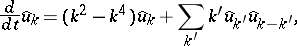
| − | The | + | The $u_{xx}$ term in (a1) is responsible for an instability at large scales; the dissipative <img align="absmiddle" border="0" src="https://www.encyclopediaofmath.org/legacyimages/k/k130/k130070/k1300708.png"/> term provides damping at small scales; and the non-linear term $uu_x$ (which has the same form as that in the Burgers or one-dimensional [[Navier–Stokes equations|Navier–Stokes equations]]) stabilizes by transferring energy between large and small scales. This is readily apparent in Fourier space, where one may write (a1) with periodic boundary conditions as |
| − | <table class="eq" style="width:100%;"> <tr><td | + | <table class="eq" style="width:100%;"> <tr><td style="width:94%;text-align:center;" valign="top"><img align="absmiddle" border="0" src="https://www.encyclopediaofmath.org/legacyimages/k/k130/k130070/k13007010.png"/></td> <td style="width:5%;text-align:right;" valign="top">(a2)</td></tr></table> |
| − | where | + | where $u ( x , t ) = i \sum _ { k } \hat { u } _ { k } ( t ) \operatorname { exp } ( i k x )$, $k = n q$, $q = 2 \pi / L$, $n \in \mathbf{Z}$, $i = \sqrt { - 1 }$. The zero solution is linearly unstable to modes with $| { k } | < 1$; these modes, whose number is proportional to the [[Bifurcation|bifurcation]] parameter $L$, are coupled to each other and to damped modes at $| { k } | > 1$ through the non-linear term. |
| − | As | + | As $L$ increases beyond $2 \pi$, therefore, the zero solution destabilizes, initially to a single-humped stationary "cellular" state, which then in turn becomes unstable through a complex hierarchy of bifurcations including multi-modal stationary, oscillatory and chaotic solutions, which have been characterized in detail [[#References|[a15]]], [[#References|[a13]]], [[#References|[a17]]]. Note that as suggested by the presence of chaotic solutions and by a Painlevé analysis [[#References|[a7]]] (cf. also [[Painlevé test|Painlevé test]]), the Kuramoto–Sivashinsky equation is non-integrable, and no explicit general analytic solutions exist. A striking feature of the bifurcation behaviour in this partial differential equation, especially for relatively small $L$, is the apparent low-dimensionality of the dynamics, and the similarity of the observed bifurcations to those found in (low) finite-dimensional systems. Motivated by this observation, extensive analytical study of the solutions has shown that the Kuramoto–Sivashinsky equation is rigorously equivalent to a finite-dimensional dynamical system (for an overview of analytical results in an appropriate functional setting, see [[#References|[a32]]]). |
==Analytical results and finite-dimensionality of dynamics.== | ==Analytical results and finite-dimensionality of dynamics.== | ||
| − | Specifically, a significant feature of the Kuramoto–Sivashinsky dynamics is its dissipativity (cf. also [[Dissipative system|Dissipative system]]): solutions are attracted to an absorbing ball, with | + | Specifically, a significant feature of the Kuramoto–Sivashinsky dynamics is its dissipativity (cf. also [[Dissipative system|Dissipative system]]): solutions are attracted to an absorbing ball, with $L$-dependent radius, in $\operatorname{L} ^ { 2 }$ and higher Sobolev spaces ([[#References|[a26]]] for odd initial data, [[#References|[a2]]], [[#References|[a12]]] for general periodic solutions; cf. also [[Sobolev space|Sobolev space]]). The strong smoothing properties of the linear operator in fact imply boundedness in the Gevrey norm (cf. [[Gevrey class|Gevrey class]]) and thus space-analyticity of solutions of (a1) [[#References|[a3]]], as well as time-analyticity [[#References|[a16]]]. |
The dissipativity of the dynamics has been used to show [[#References|[a26]]] that the system (a1) has a finite number of determining modes, and a compact global attractor with finite fractal and [[Hausdorff dimension|Hausdorff dimension]]. While the attractor can have very complex structure, a stronger result is the existence of a finite-dimensional inertial manifold, which exponentially absorbs solutions and contains the global attractor [[#References|[a10]]], [[#References|[a4]]]. On restricting the partial differential equation to the inertial manifold, one obtains a system of ordinary differential equations, the inertial form, which completely describes the long-time dynamics; thus, the Kuramoto–Sivashinsky equation is rigorously equivalent to a finite-dimensional [[Dynamical system|dynamical system]]. The existence of the inertial manifold does not provide an explicit construction, however, so various approximation schemes have been introduced; for instance, one can construct approximate inertial manifolds so that all trajectories of the Kuramoto–Sivashinsky equation approach the approximate inertial manifold at an exponential rate [[#References|[a16]]]. | The dissipativity of the dynamics has been used to show [[#References|[a26]]] that the system (a1) has a finite number of determining modes, and a compact global attractor with finite fractal and [[Hausdorff dimension|Hausdorff dimension]]. While the attractor can have very complex structure, a stronger result is the existence of a finite-dimensional inertial manifold, which exponentially absorbs solutions and contains the global attractor [[#References|[a10]]], [[#References|[a4]]]. On restricting the partial differential equation to the inertial manifold, one obtains a system of ordinary differential equations, the inertial form, which completely describes the long-time dynamics; thus, the Kuramoto–Sivashinsky equation is rigorously equivalent to a finite-dimensional [[Dynamical system|dynamical system]]. The existence of the inertial manifold does not provide an explicit construction, however, so various approximation schemes have been introduced; for instance, one can construct approximate inertial manifolds so that all trajectories of the Kuramoto–Sivashinsky equation approach the approximate inertial manifold at an exponential rate [[#References|[a16]]]. | ||
==Bifurcations and elementary solutions.== | ==Bifurcations and elementary solutions.== | ||
| − | The cellular or "roll" solutions [[#References|[a11]]] form the backbone to the spatial structure of solutions of (a1) (with periodic boundary conditions) observed as | + | The cellular or "roll" solutions [[#References|[a11]]] form the backbone to the spatial structure of solutions of (a1) (with periodic boundary conditions) observed as $L$ increases: the $N$-cell state consists of solutions with periodicity $L / N$ which lie on the branch bifurcating from the trivial solution at $L = N . 2 \pi$, and have rapidly decreasing basin of attraction for increasing $N$ [[#References|[a9]]]. Other solutions observed numerically for increasing $L$, and in some cases accounted for analytically, include other families of stationary states, time-periodic standing and travelling waves, quasi-periodic modulated travelling waves, and heteroclinic cycles [[#References|[a1]]], [[#References|[a17]]]. There are also windows in which strange attractors with positive Lyapunov exponents (cf. [[Lyapunov characteristic exponent|Lyapunov characteristic exponent]]) are observed, together with more complex dynamical phenomena associated with chaotic dynamics, including period doubling cascades, Shil'nikov connections and crises of chaos. |
==Spatio-temporal chaos.== | ==Spatio-temporal chaos.== | ||
| − | As | + | As $L$ increases and one passes through an increasingly intricate bifurcation sequence of ordered and chaotic states, eventually one reaches a state of persistent dynamical disorder for (almost) all sufficiently large $L$ [[#References|[a13]]] (see Fig.a1), and there is strong numerical evidence that the "simple" solutions destabilize to an (apparently unique) spatio-temporally chaotic attractor (see [[#References|[a8]]] for a review of spatio-temporal pattern formation). |
| − | <img | + | <img src="https://www.encyclopediaofmath.org/legacyimages/common_img/k130070a.gif" style="border:1px solid;"/> |
Figure: k130070a | Figure: k130070a | ||
| − | A solution | + | A solution $u ( x , t )$ of the Kuramoto–Sivashinsky equation (a1)on the spatio-temporally chaotic attractor, for $L = 100$, and covering $256$ time units separated by $\Delta t = 1$ |
This regime of "weak" or "phase" turbulence [[#References|[a23]]] is distinct from the "strong" turbulence exhibited in, for instance, the [[Navier–Stokes equations|Navier–Stokes equations]] for fluids, in that there are no major excursions from space or time averages. While the individual solutions bifurcating from the zero solution break the translational, parity and Galilean symmetries of (a1), the spatio-temporally chaotic state displays "re-emergent order" , in that the symmetries are restored in a statistically averaged sense. | This regime of "weak" or "phase" turbulence [[#References|[a23]]] is distinct from the "strong" turbulence exhibited in, for instance, the [[Navier–Stokes equations|Navier–Stokes equations]] for fluids, in that there are no major excursions from space or time averages. While the individual solutions bifurcating from the zero solution break the translational, parity and Galilean symmetries of (a1), the spatio-temporally chaotic state displays "re-emergent order" , in that the symmetries are restored in a statistically averaged sense. | ||
| − | Numerical evidence indicates that the spatio-temporally chaotic state is characterized by a finite density of positive Lyapunov exponents, that is, the Lyapunov dimension of the attractor is proportional to | + | Numerical evidence indicates that the spatio-temporally chaotic state is characterized by a finite density of positive Lyapunov exponents, that is, the Lyapunov dimension of the attractor is proportional to $L$ [[#References|[a22]]]. In fact, in general there appears to be "extensive chaos" for sufficiently large $L$: that is, due to rapid decay of spatial correlations [[#References|[a33]]] local dynamics are asymptotically independent of system size $L$, extensive quantities such as the energy (square of the $\operatorname{L} ^ { 2 }$ norm) scale with $L$, and one can hope to study the thermodynamic limit, interpreting the large system as being composed of weakly interacting smaller subsystems. |
| − | However, this picture is as yet by no means well-established, and even relatively "simple" analytical results on intensive properties which might seem rigorously provable, have remained elusive at the time of this writing (2000). For example, the known analytical and numerical solutions all appear to have uniformly bounded | + | However, this picture is as yet by no means well-established, and even relatively "simple" analytical results on intensive properties which might seem rigorously provable, have remained elusive at the time of this writing (2000). For example, the known analytical and numerical solutions all appear to have uniformly bounded $| u ( x , t ) |$, that is, the $\operatorname{L} ^ { \infty }$ norm $\| u \|_{\infty}$ is bounded independent of $L$; this would imply the existence of a finite energy density, or that the $\operatorname{L} ^ { 2 }$ norm |
| − | + | \begin{equation*} \| u \| _ { 2 } = \left[ \int _ { - L / 2 } ^ { L / 2 } u ^ { 2 } ( x , t ) d x \right] ^ { 1 / 2 } \end{equation*} | |
| − | is proportional to | + | is proportional to $L^{1/2}$. While a uniform bound on $\| u \|_{\infty}$ is known for stationary solutions [[#References|[a25]]] and solutions near these on the attractor, currently (2000) the best known general bound for $\| u \| _ { 2 }$ is $O ( L ^ { 8 / 5 } )$ [[#References|[a2]]]. Similarly, based on extensive numerical evidence, it has been conjectured [[#References|[a2]]], [[#References|[a27]]], [[#References|[a26]]] that the attractor and inertial manifold dimensions scale linearly with $L$, or with the number of linearly unstable Fourier modes, while the radius of the strip of space-analyticity is $L$-independent [[#References|[a3]]]; but the best known rigorous bounds for the Kuramoto–Sivashinsky equation do not yet approach this thermodynamic limit. |
| − | The dynamics on the spatio-temporally complex attractor for large | + | The dynamics on the spatio-temporally complex attractor for large $L$ are best understood in the light of the characteristic shape of the normalized (time-averaged) power spectrum <img align="absmiddle" border="0" src="https://www.encyclopediaofmath.org/legacyimages/k/k130/k130070/k13007054.png"/>, which appears to be independent of $L$ in the disordered regime, consistent with a finite energy density [[#References|[a27]]], [[#References|[a28]]] (see Fig.a2). |
| − | The power spectrum reveals three distinct regimes of the dynamics, whose dynamical significance is corroborated by other evidence including numerical experiments in which different modes are eliminated or forced [[#References|[a33]]]: The exponential tail in | + | The power spectrum reveals three distinct regimes of the dynamics, whose dynamical significance is corroborated by other evidence including numerical experiments in which different modes are eliminated or forced [[#References|[a33]]]: The exponential tail in $S ( k )$ is due to strong dissipation at small scales (high $k$), corresponding to the exponential decay of Fourier modes of an analytic function; these modes are strongly damped and essentially irrelevant for the qualitative dynamics. The active scales for $k = O ( 1 )$ have distinctly non-Gaussian distributions and contain most of the energy, with a pronounced peak near $k = 1 / \sqrt { 2 }$, the most linearly unstable mode; the localized dynamics at these scales, which may be interpreted as cell creation and annihilation events [[#References|[a6]]], are essential to the spatio-temporal disorder. |
| − | <img | + | <img src="https://www.encyclopediaofmath.org/legacyimages/common_img/k130070b.gif" style="border:1px solid;"/> |
Figure: k130070b | Figure: k130070b | ||
| − | Rescaled power spectrum | + | Rescaled power spectrum $S ( k )$, for $L = 100$ and $L = 800$ |
| − | In the large scale region, there is a shoulder in | + | In the large scale region, there is a shoulder in $S ( k )$ which flattens as $k \rightarrow 0$, reminiscent of a thermodynamic regime with equipartition of energy. These scales exhibit Gaussian statistics and appear to act as a "heat bath" , providing the background excitation needed to maintain the spatio-temporal disorder [[#References|[a33]]]. There has been considerable effort devoted towards understanding the effective stochastic dynamics at large length and time scales [[#References|[a35]]], [[#References|[a29]]], [[#References|[a20]]], [[#References|[a6]]]. The (deterministic) chaotic dynamics at active and small scales simulate the effect of random forcing on the largest scales, and act to renormalize the viscosity, so that the scaling of solutions at large scales appears to be well-described by a noise-driven Burgers equation or, equivalently, the Kardar–Parisi–Zhang equation for kinetic roughening [[#References|[a34]]], [[#References|[a18]]] (see [[#References|[a14]]] for a review). |
| − | Numerous investigators have extended the above-mentioned results on the analysis and dynamics of the Kuramoto–Sivashinsky equation in the small- | + | Numerous investigators have extended the above-mentioned results on the analysis and dynamics of the Kuramoto–Sivashinsky equation in the small-$L$ and large-$L$ regimes, and have studied generalizations to higher space dimensions and non-periodic boundary conditions (including the unbounded system, $X \in \mathbf R$), and the effect of additional terms in the partial differential equation. |
====References==== | ====References==== | ||
| − | <table>< | + | <table><tr><td valign="top">[a1]</td> <td valign="top"> D. Armbruster, J. Guckenheimer, P. Holmes, "Kuramoto–Sivashinsky dynamics on the center-unstable manifold" ''SIAM J. Appl. Math.'' , '''49''' (1989) pp. 676–691</td></tr><tr><td valign="top">[a2]</td> <td valign="top"> P. Collet, J.-P. Eckmann, H. Epstein, J. Stubbe, "A global attracting set for the Kuramoto-Sivashinsky equation" ''Commun. Math. Phys.'' , '''152''' (1993) pp. 203–214</td></tr><tr><td valign="top">[a3]</td> <td valign="top"> P. Collet, J.-P. Eckmann, H. Epstein, J. Stubbe, "Analyticity for the Kuramoto-Sivashinsky equation" ''Physica D'' , '''67''' (1993) pp. 321–326</td></tr><tr><td valign="top">[a4]</td> <td valign="top"> P. Constantin, C. Foias, B. Nicolaenko, R. Temam, "Integral manifolds and inertial manifolds for dissipative partial differential equations" , ''Appl. Math. Sci.'' , '''70''' , Springer (1989)</td></tr><tr><td valign="top">[a5]</td> <td valign="top"> B. Cohen, J. Krommes, W. Tang, M. Rosenbluth, "Nonlinear saturation of the dissipative trapped-ion mode by mode coupling" ''Nucl. Fus.'' , '''16''' (1976) pp. 971–992</td></tr><tr><td valign="top">[a6]</td> <td valign="top"> C.C. Chow, T. Hwa, "Defect-mediated stability: an effective hydrodynamic theory of spatiotemporal chaos" ''Physica D'' , '''84''' (1995) pp. 494–512</td></tr><tr><td valign="top">[a7]</td> <td valign="top"> R. Conte, M. Musette, "Painlevé analysis and Bäcklund transformation in the Kuramoto-Sivashinsky equation" ''J. Phys. A'' , '''22''' (1989) pp. 169–177</td></tr><tr><td valign="top">[a8]</td> <td valign="top"> M. Cross, P. Hohenberg, "Pattern formation outside of equilibrium" ''Rev. Mod. Phys.'' , '''65''' (1993) pp. 851–1112</td></tr><tr><td valign="top">[a9]</td> <td valign="top"> J.N. Elgin, X. Wu, "Stability of cellular states of the Kuramoto-Sivashinsky equation" ''SIAM J. Appl. Math.'' , '''56''' (1996) pp. 1621–1638</td></tr><tr><td valign="top">[a10]</td> <td valign="top"> C. Foias, B. Nicolaenko, G.R. Sell, R. Temam, "Inertial manifolds for the Kuramoto-Sivashinsky equation and an estimate of their lowest dimension" ''J. Math. Pures Appl.'' , '''67''' (1988) pp. 197–226</td></tr><tr><td valign="top">[a11]</td> <td valign="top"> U. Frisch, Z.S. She, and O. Thual, "Viscoelastic behaviour of cellular solutions to the Kuramoto-Sivashinsky model" ''J. Fluid Mech.'' , '''168''' (1986) pp. 221–240</td></tr><tr><td valign="top">[a12]</td> <td valign="top"> J. Goodman, "Stability of the Kuramoto-Sivashinsky and related systems" ''Commun. Pure Appl. Math.'' , '''47''' (1994) pp. 293–306</td></tr><tr><td valign="top">[a13]</td> <td valign="top"> J.M. Hyman, B. Nicolaenko, S. Zaleski, "Order and complexity in the Kuramoto-Sivashinsky model of weakly turbulent interfaces" ''Physica D'' , '''23''' (1986) pp. 265–292</td></tr><tr><td valign="top">[a14]</td> <td valign="top"> T. Halpin–Healy, Y.-C. Zhang, "Kinetic roughening phenomena, stochastic growth, directed polymers and all that" ''Phys. Rept.'' , '''254''' (1995) pp. 215–414</td></tr><tr><td valign="top">[a15]</td> <td valign="top"> J.M. Hyman, B. Nicolaenko, "The Kuramoto-Sivashinsky equation: A bridge between PDEs and dynamical systems" ''Physica D'' , '''18''' (1986) pp. 113–126</td></tr><tr><td valign="top">[a16]</td> <td valign="top"> M. Jolly, I. Kevrekidis, E. Titi, "Approximate inertial manifolds for the Kuramoto-Sivashinsky equation: Analysis and computation" ''Physica D'' , '''44''' (1990) pp. 38–60</td></tr><tr><td valign="top">[a17]</td> <td valign="top"> I.G. Kevrekidis, B. Nicolaenko, J.C. Scovel, "Back in the saddle again: A computer assisted study of the Kuramoto-Sivashinsky equation" ''SIAM J. Appl. Math.'' , '''50''' (1990) pp. 760–790</td></tr><tr><td valign="top">[a18]</td> <td valign="top"> M. Kardar, G. Parisi, Y.-C. Zhang, "Dynamic scaling of growing interfaces" ''Phys. Rev. Lett.'' , '''56''' (1986) pp. 889–892</td></tr><tr><td valign="top">[a19]</td> <td valign="top"> Y. Kuramoto, T. Tsuzuki, "Persistent propagation of concentration waves in dissipative media far from thermal equilibrium" ''Progr. Theoret. Phys.'' , '''55''' (1976) pp. 356–369</td></tr><tr><td valign="top">[a20]</td> <td valign="top"> V.S. L'vov, V.V. Lebedev, M. Paton, I. Procaccia, "Proof of scale invariant solutions in the Kardar–Parisi–Zhang and Kuramoto-Sivashinsky equations in $1 + 1$ dimensions: analytical and numerical results" ''Nonlinearity'' , '''6''' (1993) pp. 25–47</td></tr><tr><td valign="top">[a21]</td> <td valign="top"> R. LaQuey, S. Mahajan, P. Rutherford, W. Tang, "Nonlinear saturation of the trapped-ion mode" ''Phys. Rev. Lett.'' , '''34''' (1975) pp. 391–394</td></tr><tr><td valign="top">[a22]</td> <td valign="top"> P. Manneville, "Liapounov exponents for the Kuramoto-Sivashinsky model" U. Frisch (ed.) J. Keller (ed.) G. Papanicolaou (ed.) O. Pironneau (ed.) , ''Macroscopic Modelling of Turbulent Flows'' , ''Lecture Notes in Physics'' , '''230''' , Springer (1985) pp. 319–326</td></tr><tr><td valign="top">[a23]</td> <td valign="top"> P. Manneville, "Dissipative structures and weak turbulence" , Acad. Press (1990)</td></tr><tr><td valign="top">[a24]</td> <td valign="top"> C. Misbah, A. Valance, "Secondary instabilities in the stabilized Kuramoto-Sivashinsky equation" ''Phys. Rev. E'' , '''49''' (1994) pp. 166–183</td></tr><tr><td valign="top">[a25]</td> <td valign="top"> D. Michelson, "Steady solutions of the Kuramoto-Sivashinsky equation" ''Physica D'' , '''19''' (1986) pp. 89–111</td></tr><tr><td valign="top">[a26]</td> <td valign="top"> B. Nicolaenko, B. Scheurer, R. Temam, "Some global dynamical properties of the Kuramoto-Sivashinsky equations: Nonlinear stability and attractors" ''Physica D'' , '''16''' (1985) pp. 155–183</td></tr><tr><td valign="top">[a27]</td> <td valign="top"> Y. Pomeau, A. Pumir, P. Pelce, "Intrinsic stochasticity with many degrees of freedom" ''J. Statist. Phys.'' , '''37''' (1984) pp. 39–49</td></tr><tr><td valign="top">[a28]</td> <td valign="top"> A. Pumir, "Statistical properties of an equation describing fluid interfaces" ''J. Physique'' , '''46''' (1985) pp. 511–522</td></tr><tr><td valign="top">[a29]</td> <td valign="top"> K. Sneppen, J. Krug, M. Jensen, C. Jayaprakash, T. Bohr, "Dynamic scaling and crossover analysis for the Kuramoto-Sivashinsky equation" ''Phys. Rev. A'' , '''46''' (1992) pp. R7351–R7354</td></tr><tr><td valign="top">[a30]</td> <td valign="top"> G. Sivashinsky, D. Michelson, "On irregular wavy flow of a liquid film down a vertical plane" ''Progr. Theoret. Phys.'' , '''63''' (1980) pp. 2112–2114</td></tr><tr><td valign="top">[a31]</td> <td valign="top"> G. Sivashinsky, "Nonlinear analysis of hydrodynamic instability in laminar flames I. Derivation of basic equations" ''Acta Astron.'' , '''4''' (1977) pp. 1177–1206</td></tr><tr><td valign="top">[a32]</td> <td valign="top"> R. Temam, "Infinite-dimensional dynamical systems in mechanics and physics" , ''Applied Math. Sci.'' , '''68''' , Springer (1997) (Edition: Second)</td></tr><tr><td valign="top">[a33]</td> <td valign="top"> R.W. Wittenberg, P. Holmes, "Scale and space localization in the Kuramoto–Sivashinsky equation" ''Chaos'' , '''9''' (1999) pp. 452–465</td></tr><tr><td valign="top">[a34]</td> <td valign="top"> V. Yakhot, "Large-scale properties of unstable systems governed by the Kuramoto-Sivashinski equation" ''Phys. Rev. A'' , '''24''' (1981) pp. 642–644</td></tr><tr><td valign="top">[a35]</td> <td valign="top"> S. Zaleski, "A stochastic model for the large scale dynamics of some fluctuating interfaces" ''Physica D'' , '''34''' (1989) pp. 427–438</td></tr></table> |
Latest revision as of 17:43, 1 July 2020
Sivashinsky–Kuramoto equation, KS equation
The Kuramoto–Sivashinsky equation in one space dimension, in "derivative" form
\begin{equation} \tag{a1} u _ { t } + u _ { xxxx } + u _ { xx } + u u _ { x } = 0 , \quad x \in [ - L / 2 , L / 2 ], \end{equation}
or in "integral" form
\begin{equation*} h _ { t } + h _ { xxxx } + h _ {xx } + \frac { 1 } { 2 } h _ { x } ^ { 2 } = 0, \end{equation*}
where $u = h _ { x }$, has attracted a great deal of interest as a model for complex spatio-temporal dynamics in spatially extended systems, and as a paradigm for finite-dimensional dynamics in a partial differential equation.
The Kuramoto–Sivashinsky equation (with various alternative scalings for $u$, $x$ or $t$, which can be reduced to the form (a1)) has been independently derived in the context of several extended physical systems driven far from equilibrium by intrinsic instabilities, including instabilities of dissipative trapped ion modes in plasmas [a21], [a5], instabilities in laminar flame fronts [a31], phase dynamics in reaction-diffusion systems [a19], and fluctuations in fluid films on inclines [a30]. Indeed, (a1) generically describes the dynamics near long-wave-length primary instabilities in the presence of appropriate (translational, parity and Galilean) symmetries [a24].
The $u_{xx}$ term in (a1) is responsible for an instability at large scales; the dissipative  term provides damping at small scales; and the non-linear term $uu_x$ (which has the same form as that in the Burgers or one-dimensional Navier–Stokes equations) stabilizes by transferring energy between large and small scales. This is readily apparent in Fourier space, where one may write (a1) with periodic boundary conditions as
 | (a2) |
where $u ( x , t ) = i \sum _ { k } \hat { u } _ { k } ( t ) \operatorname { exp } ( i k x )$, $k = n q$, $q = 2 \pi / L$, $n \in \mathbf{Z}$, $i = \sqrt { - 1 }$. The zero solution is linearly unstable to modes with $| { k } | < 1$; these modes, whose number is proportional to the bifurcation parameter $L$, are coupled to each other and to damped modes at $| { k } | > 1$ through the non-linear term.
As $L$ increases beyond $2 \pi$, therefore, the zero solution destabilizes, initially to a single-humped stationary "cellular" state, which then in turn becomes unstable through a complex hierarchy of bifurcations including multi-modal stationary, oscillatory and chaotic solutions, which have been characterized in detail [a15], [a13], [a17]. Note that as suggested by the presence of chaotic solutions and by a Painlevé analysis [a7] (cf. also Painlevé test), the Kuramoto–Sivashinsky equation is non-integrable, and no explicit general analytic solutions exist. A striking feature of the bifurcation behaviour in this partial differential equation, especially for relatively small $L$, is the apparent low-dimensionality of the dynamics, and the similarity of the observed bifurcations to those found in (low) finite-dimensional systems. Motivated by this observation, extensive analytical study of the solutions has shown that the Kuramoto–Sivashinsky equation is rigorously equivalent to a finite-dimensional dynamical system (for an overview of analytical results in an appropriate functional setting, see [a32]).
Analytical results and finite-dimensionality of dynamics.
Specifically, a significant feature of the Kuramoto–Sivashinsky dynamics is its dissipativity (cf. also Dissipative system): solutions are attracted to an absorbing ball, with $L$-dependent radius, in $\operatorname{L} ^ { 2 }$ and higher Sobolev spaces ([a26] for odd initial data, [a2], [a12] for general periodic solutions; cf. also Sobolev space). The strong smoothing properties of the linear operator in fact imply boundedness in the Gevrey norm (cf. Gevrey class) and thus space-analyticity of solutions of (a1) [a3], as well as time-analyticity [a16].
The dissipativity of the dynamics has been used to show [a26] that the system (a1) has a finite number of determining modes, and a compact global attractor with finite fractal and Hausdorff dimension. While the attractor can have very complex structure, a stronger result is the existence of a finite-dimensional inertial manifold, which exponentially absorbs solutions and contains the global attractor [a10], [a4]. On restricting the partial differential equation to the inertial manifold, one obtains a system of ordinary differential equations, the inertial form, which completely describes the long-time dynamics; thus, the Kuramoto–Sivashinsky equation is rigorously equivalent to a finite-dimensional dynamical system. The existence of the inertial manifold does not provide an explicit construction, however, so various approximation schemes have been introduced; for instance, one can construct approximate inertial manifolds so that all trajectories of the Kuramoto–Sivashinsky equation approach the approximate inertial manifold at an exponential rate [a16].
Bifurcations and elementary solutions.
The cellular or "roll" solutions [a11] form the backbone to the spatial structure of solutions of (a1) (with periodic boundary conditions) observed as $L$ increases: the $N$-cell state consists of solutions with periodicity $L / N$ which lie on the branch bifurcating from the trivial solution at $L = N . 2 \pi$, and have rapidly decreasing basin of attraction for increasing $N$ [a9]. Other solutions observed numerically for increasing $L$, and in some cases accounted for analytically, include other families of stationary states, time-periodic standing and travelling waves, quasi-periodic modulated travelling waves, and heteroclinic cycles [a1], [a17]. There are also windows in which strange attractors with positive Lyapunov exponents (cf. Lyapunov characteristic exponent) are observed, together with more complex dynamical phenomena associated with chaotic dynamics, including period doubling cascades, Shil'nikov connections and crises of chaos.
Spatio-temporal chaos.
As $L$ increases and one passes through an increasingly intricate bifurcation sequence of ordered and chaotic states, eventually one reaches a state of persistent dynamical disorder for (almost) all sufficiently large $L$ [a13] (see Fig.a1), and there is strong numerical evidence that the "simple" solutions destabilize to an (apparently unique) spatio-temporally chaotic attractor (see [a8] for a review of spatio-temporal pattern formation).
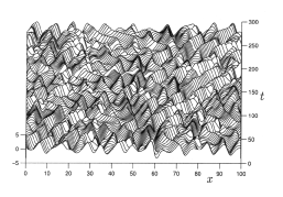
Figure: k130070a
A solution $u ( x , t )$ of the Kuramoto–Sivashinsky equation (a1)on the spatio-temporally chaotic attractor, for $L = 100$, and covering $256$ time units separated by $\Delta t = 1$
This regime of "weak" or "phase" turbulence [a23] is distinct from the "strong" turbulence exhibited in, for instance, the Navier–Stokes equations for fluids, in that there are no major excursions from space or time averages. While the individual solutions bifurcating from the zero solution break the translational, parity and Galilean symmetries of (a1), the spatio-temporally chaotic state displays "re-emergent order" , in that the symmetries are restored in a statistically averaged sense.
Numerical evidence indicates that the spatio-temporally chaotic state is characterized by a finite density of positive Lyapunov exponents, that is, the Lyapunov dimension of the attractor is proportional to $L$ [a22]. In fact, in general there appears to be "extensive chaos" for sufficiently large $L$: that is, due to rapid decay of spatial correlations [a33] local dynamics are asymptotically independent of system size $L$, extensive quantities such as the energy (square of the $\operatorname{L} ^ { 2 }$ norm) scale with $L$, and one can hope to study the thermodynamic limit, interpreting the large system as being composed of weakly interacting smaller subsystems.
However, this picture is as yet by no means well-established, and even relatively "simple" analytical results on intensive properties which might seem rigorously provable, have remained elusive at the time of this writing (2000). For example, the known analytical and numerical solutions all appear to have uniformly bounded $| u ( x , t ) |$, that is, the $\operatorname{L} ^ { \infty }$ norm $\| u \|_{\infty}$ is bounded independent of $L$; this would imply the existence of a finite energy density, or that the $\operatorname{L} ^ { 2 }$ norm
\begin{equation*} \| u \| _ { 2 } = \left[ \int _ { - L / 2 } ^ { L / 2 } u ^ { 2 } ( x , t ) d x \right] ^ { 1 / 2 } \end{equation*}
is proportional to $L^{1/2}$. While a uniform bound on $\| u \|_{\infty}$ is known for stationary solutions [a25] and solutions near these on the attractor, currently (2000) the best known general bound for $\| u \| _ { 2 }$ is $O ( L ^ { 8 / 5 } )$ [a2]. Similarly, based on extensive numerical evidence, it has been conjectured [a2], [a27], [a26] that the attractor and inertial manifold dimensions scale linearly with $L$, or with the number of linearly unstable Fourier modes, while the radius of the strip of space-analyticity is $L$-independent [a3]; but the best known rigorous bounds for the Kuramoto–Sivashinsky equation do not yet approach this thermodynamic limit.
The dynamics on the spatio-temporally complex attractor for large $L$ are best understood in the light of the characteristic shape of the normalized (time-averaged) power spectrum 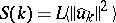 , which appears to be independent of $L$ in the disordered regime, consistent with a finite energy density [a27], [a28] (see Fig.a2).
The power spectrum reveals three distinct regimes of the dynamics, whose dynamical significance is corroborated by other evidence including numerical experiments in which different modes are eliminated or forced [a33]: The exponential tail in $S ( k )$ is due to strong dissipation at small scales (high $k$), corresponding to the exponential decay of Fourier modes of an analytic function; these modes are strongly damped and essentially irrelevant for the qualitative dynamics. The active scales for $k = O ( 1 )$ have distinctly non-Gaussian distributions and contain most of the energy, with a pronounced peak near $k = 1 / \sqrt { 2 }$, the most linearly unstable mode; the localized dynamics at these scales, which may be interpreted as cell creation and annihilation events [a6], are essential to the spatio-temporal disorder.

Figure: k130070b
Rescaled power spectrum $S ( k )$, for $L = 100$ and $L = 800$
In the large scale region, there is a shoulder in $S ( k )$ which flattens as $k \rightarrow 0$, reminiscent of a thermodynamic regime with equipartition of energy. These scales exhibit Gaussian statistics and appear to act as a "heat bath" , providing the background excitation needed to maintain the spatio-temporal disorder [a33]. There has been considerable effort devoted towards understanding the effective stochastic dynamics at large length and time scales [a35], [a29], [a20], [a6]. The (deterministic) chaotic dynamics at active and small scales simulate the effect of random forcing on the largest scales, and act to renormalize the viscosity, so that the scaling of solutions at large scales appears to be well-described by a noise-driven Burgers equation or, equivalently, the Kardar–Parisi–Zhang equation for kinetic roughening [a34], [a18] (see [a14] for a review).
Numerous investigators have extended the above-mentioned results on the analysis and dynamics of the Kuramoto–Sivashinsky equation in the small-$L$ and large-$L$ regimes, and have studied generalizations to higher space dimensions and non-periodic boundary conditions (including the unbounded system, $X \in \mathbf R$), and the effect of additional terms in the partial differential equation.
References
| [a1] | D. Armbruster, J. Guckenheimer, P. Holmes, "Kuramoto–Sivashinsky dynamics on the center-unstable manifold" SIAM J. Appl. Math. , 49 (1989) pp. 676–691 |
| [a2] | P. Collet, J.-P. Eckmann, H. Epstein, J. Stubbe, "A global attracting set for the Kuramoto-Sivashinsky equation" Commun. Math. Phys. , 152 (1993) pp. 203–214 |
| [a3] | P. Collet, J.-P. Eckmann, H. Epstein, J. Stubbe, "Analyticity for the Kuramoto-Sivashinsky equation" Physica D , 67 (1993) pp. 321–326 |
| [a4] | P. Constantin, C. Foias, B. Nicolaenko, R. Temam, "Integral manifolds and inertial manifolds for dissipative partial differential equations" , Appl. Math. Sci. , 70 , Springer (1989) |
| [a5] | B. Cohen, J. Krommes, W. Tang, M. Rosenbluth, "Nonlinear saturation of the dissipative trapped-ion mode by mode coupling" Nucl. Fus. , 16 (1976) pp. 971–992 |
| [a6] | C.C. Chow, T. Hwa, "Defect-mediated stability: an effective hydrodynamic theory of spatiotemporal chaos" Physica D , 84 (1995) pp. 494–512 |
| [a7] | R. Conte, M. Musette, "Painlevé analysis and Bäcklund transformation in the Kuramoto-Sivashinsky equation" J. Phys. A , 22 (1989) pp. 169–177 |
| [a8] | M. Cross, P. Hohenberg, "Pattern formation outside of equilibrium" Rev. Mod. Phys. , 65 (1993) pp. 851–1112 |
| [a9] | J.N. Elgin, X. Wu, "Stability of cellular states of the Kuramoto-Sivashinsky equation" SIAM J. Appl. Math. , 56 (1996) pp. 1621–1638 |
| [a10] | C. Foias, B. Nicolaenko, G.R. Sell, R. Temam, "Inertial manifolds for the Kuramoto-Sivashinsky equation and an estimate of their lowest dimension" J. Math. Pures Appl. , 67 (1988) pp. 197–226 |
| [a11] | U. Frisch, Z.S. She, and O. Thual, "Viscoelastic behaviour of cellular solutions to the Kuramoto-Sivashinsky model" J. Fluid Mech. , 168 (1986) pp. 221–240 |
| [a12] | J. Goodman, "Stability of the Kuramoto-Sivashinsky and related systems" Commun. Pure Appl. Math. , 47 (1994) pp. 293–306 |
| [a13] | J.M. Hyman, B. Nicolaenko, S. Zaleski, "Order and complexity in the Kuramoto-Sivashinsky model of weakly turbulent interfaces" Physica D , 23 (1986) pp. 265–292 |
| [a14] | T. Halpin–Healy, Y.-C. Zhang, "Kinetic roughening phenomena, stochastic growth, directed polymers and all that" Phys. Rept. , 254 (1995) pp. 215–414 |
| [a15] | J.M. Hyman, B. Nicolaenko, "The Kuramoto-Sivashinsky equation: A bridge between PDEs and dynamical systems" Physica D , 18 (1986) pp. 113–126 |
| [a16] | M. Jolly, I. Kevrekidis, E. Titi, "Approximate inertial manifolds for the Kuramoto-Sivashinsky equation: Analysis and computation" Physica D , 44 (1990) pp. 38–60 |
| [a17] | I.G. Kevrekidis, B. Nicolaenko, J.C. Scovel, "Back in the saddle again: A computer assisted study of the Kuramoto-Sivashinsky equation" SIAM J. Appl. Math. , 50 (1990) pp. 760–790 |
| [a18] | M. Kardar, G. Parisi, Y.-C. Zhang, "Dynamic scaling of growing interfaces" Phys. Rev. Lett. , 56 (1986) pp. 889–892 |
| [a19] | Y. Kuramoto, T. Tsuzuki, "Persistent propagation of concentration waves in dissipative media far from thermal equilibrium" Progr. Theoret. Phys. , 55 (1976) pp. 356–369 |
| [a20] | V.S. L'vov, V.V. Lebedev, M. Paton, I. Procaccia, "Proof of scale invariant solutions in the Kardar–Parisi–Zhang and Kuramoto-Sivashinsky equations in $1 + 1$ dimensions: analytical and numerical results" Nonlinearity , 6 (1993) pp. 25–47 |
| [a21] | R. LaQuey, S. Mahajan, P. Rutherford, W. Tang, "Nonlinear saturation of the trapped-ion mode" Phys. Rev. Lett. , 34 (1975) pp. 391–394 |
| [a22] | P. Manneville, "Liapounov exponents for the Kuramoto-Sivashinsky model" U. Frisch (ed.) J. Keller (ed.) G. Papanicolaou (ed.) O. Pironneau (ed.) , Macroscopic Modelling of Turbulent Flows , Lecture Notes in Physics , 230 , Springer (1985) pp. 319–326 |
| [a23] | P. Manneville, "Dissipative structures and weak turbulence" , Acad. Press (1990) |
| [a24] | C. Misbah, A. Valance, "Secondary instabilities in the stabilized Kuramoto-Sivashinsky equation" Phys. Rev. E , 49 (1994) pp. 166–183 |
| [a25] | D. Michelson, "Steady solutions of the Kuramoto-Sivashinsky equation" Physica D , 19 (1986) pp. 89–111 |
| [a26] | B. Nicolaenko, B. Scheurer, R. Temam, "Some global dynamical properties of the Kuramoto-Sivashinsky equations: Nonlinear stability and attractors" Physica D , 16 (1985) pp. 155–183 |
| [a27] | Y. Pomeau, A. Pumir, P. Pelce, "Intrinsic stochasticity with many degrees of freedom" J. Statist. Phys. , 37 (1984) pp. 39–49 |
| [a28] | A. Pumir, "Statistical properties of an equation describing fluid interfaces" J. Physique , 46 (1985) pp. 511–522 |
| [a29] | K. Sneppen, J. Krug, M. Jensen, C. Jayaprakash, T. Bohr, "Dynamic scaling and crossover analysis for the Kuramoto-Sivashinsky equation" Phys. Rev. A , 46 (1992) pp. R7351–R7354 |
| [a30] | G. Sivashinsky, D. Michelson, "On irregular wavy flow of a liquid film down a vertical plane" Progr. Theoret. Phys. , 63 (1980) pp. 2112–2114 |
| [a31] | G. Sivashinsky, "Nonlinear analysis of hydrodynamic instability in laminar flames I. Derivation of basic equations" Acta Astron. , 4 (1977) pp. 1177–1206 |
| [a32] | R. Temam, "Infinite-dimensional dynamical systems in mechanics and physics" , Applied Math. Sci. , 68 , Springer (1997) (Edition: Second) |
| [a33] | R.W. Wittenberg, P. Holmes, "Scale and space localization in the Kuramoto–Sivashinsky equation" Chaos , 9 (1999) pp. 452–465 |
| [a34] | V. Yakhot, "Large-scale properties of unstable systems governed by the Kuramoto-Sivashinski equation" Phys. Rev. A , 24 (1981) pp. 642–644 |
| [a35] | S. Zaleski, "A stochastic model for the large scale dynamics of some fluctuating interfaces" Physica D , 34 (1989) pp. 427–438 |
Kuramoto-Sivashinsky equation. Encyclopedia of Mathematics. URL: http://encyclopediaofmath.org/index.php?title=Kuramoto-Sivashinsky_equation&oldid=13525