Difference between revisions of "Descriptive geometry"
(Importing text file) |
m (OldImage template added) |
||
| (One intermediate revision by one other user not shown) | |||
| Line 1: | Line 1: | ||
| + | <!-- | ||
| + | d0313701.png | ||
| + | $#A+1 = 19 n = 0 | ||
| + | $#C+1 = 19 : ~/encyclopedia/old_files/data/D031/D.0301370 Descriptive geometry | ||
| + | Automatically converted into TeX, above some diagnostics. | ||
| + | Please remove this comment and the {{TEX|auto}} line below, | ||
| + | if TeX found to be correct. | ||
| + | --> | ||
| + | |||
| + | {{TEX|auto}} | ||
| + | {{TEX|done}} | ||
| + | |||
A branch of geometry in which three-dimensional figures, as well as methods for solving and investigating three-dimensional problems, are studied by representing them in the plane. Such representations are constructed by means of central or parallel [[Projection|projection]] of the figure (nature, an object, an original) on the plane of projection. | A branch of geometry in which three-dimensional figures, as well as methods for solving and investigating three-dimensional problems, are studied by representing them in the plane. Such representations are constructed by means of central or parallel [[Projection|projection]] of the figure (nature, an object, an original) on the plane of projection. | ||
| Line 5: | Line 17: | ||
Figure: d031370a | Figure: d031370a | ||
| − | The most widespread kind of technical drawing is the composite drawing, constructed by means of an orthogonal projection. Essentially, the procedure is as follows. Choose two mutually perpendicular projection planes, | + | The most widespread kind of technical drawing is the composite drawing, constructed by means of an orthogonal projection. Essentially, the procedure is as follows. Choose two mutually perpendicular projection planes, $ \Pi _ {1} $ |
| + | and $ \Pi _ {2} $. | ||
| + | The plane $ \Pi _ {1} $ | ||
| + | is called the horizontal projection plane, and $ \Pi _ {2} $ | ||
| + | is the frontal projection plane. Project an arbitrary point $ A $ | ||
| + | in space orthogonally onto these planes (see Fig. a); this gives the horizontal projection $ A _ {1} $ | ||
| + | and the frontal projection $ A _ {2} $. | ||
| + | It is sometimes useful to add a third — the profile projection $ A _ {3} $ | ||
| + | on the profile plane $ \Pi _ {3} $, | ||
| + | perpendicular to $ \Pi _ {1} $ | ||
| + | and $ \Pi _ {2} $. | ||
| + | To obtain a composite drawing, combining these three projections, make the planes $ \Pi _ {1} $ | ||
| + | and $ \Pi _ {3} $ | ||
| + | coincide with $ \Pi _ {2} $( | ||
| + | the "principal" plane) by rotating them about the lines $ p _ {12} $ | ||
| + | and $ p _ {23} $ | ||
| + | in which they intersect $ \Pi _ {2} $( | ||
| + | see Fig. b). In practice, the position of the projection axes $ p _ {12} $ | ||
| + | and $ p _ {13} $ | ||
| + | is usually not marked, i.e. the position of the projection planes is defined only up to a parallel motion. | ||
<img style="border:1px solid;" src="https://www.encyclopediaofmath.org/legacyimages/common_img/d031370b.gif" /> | <img style="border:1px solid;" src="https://www.encyclopediaofmath.org/legacyimages/common_img/d031370b.gif" /> | ||
| Line 12: | Line 43: | ||
For the construction of more readily visualizable representations, descriptive geometry makes use of an [[Axonometry|axonometry]]. To represent objects of considerable extension, one uses drawings obtained by central projection — in other words, in perspective. | For the construction of more readily visualizable representations, descriptive geometry makes use of an [[Axonometry|axonometry]]. To represent objects of considerable extension, one uses drawings obtained by central projection — in other words, in perspective. | ||
| − | |||
| − | |||
| − | |||
| − | |||
| Line 24: | Line 51: | ||
====References==== | ====References==== | ||
| − | <table><TR><TD valign="top">[a1]</TD> <TD valign="top"> F. Rehbock, "Darstellende Geometrie" , Springer (1969)</TD></TR><TR><TD valign="top">[a2]</TD> <TD valign="top"> B. Leighton Wellman, "Technical descriptive geometry" , McGraw-Hill (1957)</TD></TR><TR><TD valign="top">[a3]</TD> <TD valign="top"> M. Bret, "Images de synthèse. Méthodes et algorithmes pour la réalisation d'images numériques" , Dunod (1988)</TD></TR><TR><TD valign="top">[a4]</TD> <TD valign="top"> M.A. Penna, R.R. Patterson, "Projective geometry and its applications to computer graphics" , Prentice-Hall (1986)</TD></TR></table> | + | <table><TR><TD valign="top">[1]</TD> <TD valign="top"> G. Monge, "Géométrie descriptive" , Paris (1820)</TD></TR><TR><TD valign="top">[2]</TD> <TD valign="top"> N.A. Glagolev, "Descriptive geometry" , Moscow (1953) (In Russian)</TD></TR><TR><TD valign="top">[3]</TD> <TD valign="top"> , ''A course of descriptive geometry'' , Moscow (1956)</TD></TR><TR><TD valign="top">[a1]</TD> <TD valign="top"> F. Rehbock, "Darstellende Geometrie" , Springer (1969)</TD></TR><TR><TD valign="top">[a2]</TD> <TD valign="top"> B. Leighton Wellman, "Technical descriptive geometry" , McGraw-Hill (1957)</TD></TR><TR><TD valign="top">[a3]</TD> <TD valign="top"> M. Bret, "Images de synthèse. Méthodes et algorithmes pour la réalisation d'images numériques" , Dunod (1988)</TD></TR><TR><TD valign="top">[a4]</TD> <TD valign="top"> M.A. Penna, R.R. Patterson, "Projective geometry and its applications to computer graphics" , Prentice-Hall (1986)</TD></TR></table> |
| + | |||
| + | {{OldImage}} | ||
Latest revision as of 11:38, 26 March 2023
A branch of geometry in which three-dimensional figures, as well as methods for solving and investigating three-dimensional problems, are studied by representing them in the plane. Such representations are constructed by means of central or parallel projection of the figure (nature, an object, an original) on the plane of projection.

Figure: d031370a
The most widespread kind of technical drawing is the composite drawing, constructed by means of an orthogonal projection. Essentially, the procedure is as follows. Choose two mutually perpendicular projection planes, $ \Pi _ {1} $ and $ \Pi _ {2} $. The plane $ \Pi _ {1} $ is called the horizontal projection plane, and $ \Pi _ {2} $ is the frontal projection plane. Project an arbitrary point $ A $ in space orthogonally onto these planes (see Fig. a); this gives the horizontal projection $ A _ {1} $ and the frontal projection $ A _ {2} $. It is sometimes useful to add a third — the profile projection $ A _ {3} $ on the profile plane $ \Pi _ {3} $, perpendicular to $ \Pi _ {1} $ and $ \Pi _ {2} $. To obtain a composite drawing, combining these three projections, make the planes $ \Pi _ {1} $ and $ \Pi _ {3} $ coincide with $ \Pi _ {2} $( the "principal" plane) by rotating them about the lines $ p _ {12} $ and $ p _ {23} $ in which they intersect $ \Pi _ {2} $( see Fig. b). In practice, the position of the projection axes $ p _ {12} $ and $ p _ {13} $ is usually not marked, i.e. the position of the projection planes is defined only up to a parallel motion.
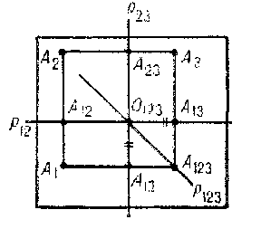
Figure: d031370b
For the construction of more readily visualizable representations, descriptive geometry makes use of an axonometry. To represent objects of considerable extension, one uses drawings obtained by central projection — in other words, in perspective.
Comments
There are many books on descriptive geometry in the German language, e.g. [a1]. An English language reference is [a2].
A renaissance of descriptive geometry has been sparked by computer graphics; e.g., in matters concerning the two-dimensional graphical representation of three-dimensional objects (perspective, hidden outlines), cf., e.g., [a3], [a4] and references therein.
References
| [1] | G. Monge, "Géométrie descriptive" , Paris (1820) |
| [2] | N.A. Glagolev, "Descriptive geometry" , Moscow (1953) (In Russian) |
| [3] | , A course of descriptive geometry , Moscow (1956) |
| [a1] | F. Rehbock, "Darstellende Geometrie" , Springer (1969) |
| [a2] | B. Leighton Wellman, "Technical descriptive geometry" , McGraw-Hill (1957) |
| [a3] | M. Bret, "Images de synthèse. Méthodes et algorithmes pour la réalisation d'images numériques" , Dunod (1988) |
| [a4] | M.A. Penna, R.R. Patterson, "Projective geometry and its applications to computer graphics" , Prentice-Hall (1986) |
Descriptive geometry. Encyclopedia of Mathematics. URL: http://encyclopediaofmath.org/index.php?title=Descriptive_geometry&oldid=16046