Difference between revisions of "Asymmetry coefficient"
(Importing text file) |
Ulf Rehmann (talk | contribs) m (tex encoded by computer) |
||
| Line 1: | Line 1: | ||
| + | <!-- | ||
| + | a0135901.png | ||
| + | $#A+1 = 29 n = 0 | ||
| + | $#C+1 = 29 : ~/encyclopedia/old_files/data/A013/A.0103590 Asymmetry coefficient | ||
| + | Automatically converted into TeX, above some diagnostics. | ||
| + | Please remove this comment and the {{TEX|auto}} line below, | ||
| + | if TeX found to be correct. | ||
| + | --> | ||
| + | |||
| + | {{TEX|auto}} | ||
| + | {{TEX|done}} | ||
| + | |||
The most frequently employed measure of the [[Asymmetry of a distribution|asymmetry of a distribution]], defined by the relationship | The most frequently employed measure of the [[Asymmetry of a distribution|asymmetry of a distribution]], defined by the relationship | ||
| − | + | $$ | |
| + | \gamma _ {1} = \mu _ | ||
| + | \frac{3}{\mu _ {2} ^ {3/2} } | ||
| + | , | ||
| + | $$ | ||
| − | where | + | where $ \mu _ {2} $ |
| + | and $ \mu _ {3} $ | ||
| + | are the second and third central moments of the distribution, respectively. For distributions that are symmetric with respect to the mathematical expectation, $ \gamma _ {1} = 0 $; | ||
| + | depending on the sign of $ \gamma _ {1} $ | ||
| + | one speaks of positive asymmetry ( $ \gamma _ {1} > 0 $) | ||
| + | and negative asymmetry ( $ \gamma _ {1} < 0 $). | ||
| + | In the case of the [[Binomial distribution|binomial distribution]] corresponding to $ n $[[ | ||
| + | Bernoulli trials|Bernoulli trials]] with probability of success $ p $, | ||
| − | + | $$ \tag{* } | |
| + | \gamma _ {1} = {%1 - 2 p } over | ||
| + | \sqrt {np ( 1 - p ) } , | ||
| + | $$ | ||
| − | one has: If | + | one has: If $ p = 1/2 ( \gamma _ {1} = 0 ) $, |
| + | the distribution is symmetric; if $ p < 1/2 $ | ||
| + | or $ p > 1/2 $, | ||
| + | one obtains typical distribution diagrams with a positive (Fig.a) and negative (Fig.b) asymmetry. | ||
<img style="border:1px solid;" src="https://www.encyclopediaofmath.org/legacyimages/common_img/a013590a.gif" /> | <img style="border:1px solid;" src="https://www.encyclopediaofmath.org/legacyimages/common_img/a013590a.gif" /> | ||
| Line 13: | Line 42: | ||
Figure: a013590a | Figure: a013590a | ||
| − | + | $ P(k, 10, 1/5 ) $. | |
| + | Diagram of the binomial distribution $ P(k, n, p) $ | ||
| + | corresponding to $ n = 10 $ | ||
| + | Bernoulli trials, with positive asymmetry ( $ p = 1/5 $). | ||
<img style="border:1px solid;" src="https://www.encyclopediaofmath.org/legacyimages/common_img/a013590b.gif" /> | <img style="border:1px solid;" src="https://www.encyclopediaofmath.org/legacyimages/common_img/a013590b.gif" /> | ||
| Line 19: | Line 51: | ||
Figure: a013590b | Figure: a013590b | ||
| − | + | $ P(k, 10, 4/5 ) $. | |
| + | Diagram of the binomial distribution $ P(k, n, p) $ | ||
| + | corresponding to $ n = 10 $ | ||
| + | Bernoulli trials, with negative asymmetry ( $ p = 4/5 $). | ||
| + | |||
| + | The asymmetry coefficient (*) tends to zero as $ n \rightarrow \infty $, | ||
| + | in accordance with the fact that a normalized binomial distribution converges to the standard normal distribution. | ||
| − | The asymmetry coefficient ( | + | The asymmetry coefficient and the [[Excess coefficient|excess coefficient]] are the most extensively used characteristics of the accuracy with which the distribution function $ F _ {n} (x) $ |
| + | of the normalized sum | ||
| − | + | $$ | |
| − | + | \frac{( X _ {1} + \dots + X _ {n} ) - n \mu _ {1} } \sqrt | |
| + | {n \mu _ {2} } , | ||
| + | $$ | ||
| − | where | + | where $ X _ {1} \dots X _ {n} $ |
| + | are identically distributed and mutually independent with asymmetry coefficient $ \delta _ {1} $, | ||
| + | may be approximated by the normal distribution function | ||
| − | + | $$ | |
| + | \Phi (x) = | ||
| + | \frac{1} \sqrt | ||
| + | {2 \pi } \int\limits _ {- \infty } ^ { x } | ||
| + | e ^ {-z ^ {2} /2 } dz . | ||
| + | $$ | ||
Under fairly general conditions the [[Edgeworth series|Edgeworth series]] yields | Under fairly general conditions the [[Edgeworth series|Edgeworth series]] yields | ||
| − | + | $$ | |
| + | F _ {n} (x) = \Phi (x) - | ||
| + | \frac{1} \sqrt | ||
| + | n \gamma _ | ||
| + | \frac{1}{6} | ||
| + | |||
| + | \Phi ^ {(3)} (x) + O \left ( | ||
| + | \frac{1}{n} | ||
| + | \right ) , | ||
| + | $$ | ||
| − | where | + | where $ \Phi ^ {(3)} (x) $ |
| + | is the derivative of order three. | ||
====References==== | ====References==== | ||
<table><TR><TD valign="top">[1]</TD> <TD valign="top"> H. Cramér, "Mathematical methods of statistics" , Princeton Univ. Press (1946)</TD></TR><TR><TD valign="top">[2]</TD> <TD valign="top"> S.S. Wilks, "Mathematical statistics" , Wiley (1962)</TD></TR></table> | <table><TR><TD valign="top">[1]</TD> <TD valign="top"> H. Cramér, "Mathematical methods of statistics" , Princeton Univ. Press (1946)</TD></TR><TR><TD valign="top">[2]</TD> <TD valign="top"> S.S. Wilks, "Mathematical statistics" , Wiley (1962)</TD></TR></table> | ||
| − | |||
| − | |||
====Comments==== | ====Comments==== | ||
Revision as of 18:48, 5 April 2020
The most frequently employed measure of the asymmetry of a distribution, defined by the relationship
$$ \gamma _ {1} = \mu _ \frac{3}{\mu _ {2} ^ {3/2} } , $$
where $ \mu _ {2} $ and $ \mu _ {3} $ are the second and third central moments of the distribution, respectively. For distributions that are symmetric with respect to the mathematical expectation, $ \gamma _ {1} = 0 $; depending on the sign of $ \gamma _ {1} $ one speaks of positive asymmetry ( $ \gamma _ {1} > 0 $) and negative asymmetry ( $ \gamma _ {1} < 0 $). In the case of the binomial distribution corresponding to $ n $[[ Bernoulli trials|Bernoulli trials]] with probability of success $ p $,
$$ \tag{* } \gamma _ {1} = {%1 - 2 p } over \sqrt {np ( 1 - p ) } , $$
one has: If $ p = 1/2 ( \gamma _ {1} = 0 ) $, the distribution is symmetric; if $ p < 1/2 $ or $ p > 1/2 $, one obtains typical distribution diagrams with a positive (Fig.a) and negative (Fig.b) asymmetry.
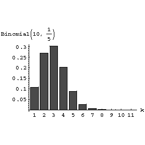
Figure: a013590a
$ P(k, 10, 1/5 ) $. Diagram of the binomial distribution $ P(k, n, p) $ corresponding to $ n = 10 $ Bernoulli trials, with positive asymmetry ( $ p = 1/5 $).

Figure: a013590b
$ P(k, 10, 4/5 ) $. Diagram of the binomial distribution $ P(k, n, p) $ corresponding to $ n = 10 $ Bernoulli trials, with negative asymmetry ( $ p = 4/5 $).
The asymmetry coefficient (*) tends to zero as $ n \rightarrow \infty $, in accordance with the fact that a normalized binomial distribution converges to the standard normal distribution.
The asymmetry coefficient and the excess coefficient are the most extensively used characteristics of the accuracy with which the distribution function $ F _ {n} (x) $ of the normalized sum
$$ \frac{( X _ {1} + \dots + X _ {n} ) - n \mu _ {1} } \sqrt {n \mu _ {2} } , $$
where $ X _ {1} \dots X _ {n} $ are identically distributed and mutually independent with asymmetry coefficient $ \delta _ {1} $, may be approximated by the normal distribution function
$$ \Phi (x) = \frac{1} \sqrt {2 \pi } \int\limits _ {- \infty } ^ { x } e ^ {-z ^ {2} /2 } dz . $$
Under fairly general conditions the Edgeworth series yields
$$ F _ {n} (x) = \Phi (x) - \frac{1} \sqrt n \gamma _ \frac{1}{6} \Phi ^ {(3)} (x) + O \left ( \frac{1}{n} \right ) , $$
where $ \Phi ^ {(3)} (x) $ is the derivative of order three.
References
| [1] | H. Cramér, "Mathematical methods of statistics" , Princeton Univ. Press (1946) |
| [2] | S.S. Wilks, "Mathematical statistics" , Wiley (1962) |
Comments
The asymmetry coefficient is usually called the coefficient of skewness. One correspondingly speaks of the skewness of a distribution and of positive, respectively negative, skewness.
The excess coefficient is more often called the coefficient of kurtosis.
Asymmetry coefficient. Encyclopedia of Mathematics. URL: http://encyclopediaofmath.org/index.php?title=Asymmetry_coefficient&oldid=45233