Difference between revisions of "Abstract wave equation"
(Importing text file) |
m (AUTOMATIC EDIT (latexlist): Replaced 77 formulas out of 79 by TEX code with an average confidence of 2.0 and a minimal confidence of 2.0.) |
||
| Line 1: | Line 1: | ||
| + | <!--This article has been texified automatically. Since there was no Nroff source code for this article, | ||
| + | the semi-automatic procedure described at https://encyclopediaofmath.org/wiki/User:Maximilian_Janisch/latexlist | ||
| + | was used. | ||
| + | If the TeX and formula formatting is correct, please remove this message and the {{TEX|semi-auto}} category. | ||
| + | |||
| + | Out of 79 formulas, 77 were replaced by TEX code.--> | ||
| + | |||
| + | {{TEX|semi-auto}}{{TEX|partial}} | ||
Consider the [[Cauchy problem|Cauchy problem]] for the [[Wave equation|wave equation]] | Consider the [[Cauchy problem|Cauchy problem]] for the [[Wave equation|wave equation]] | ||
| − | <table class="eq" style="width:100%;"> <tr><td | + | <table class="eq" style="width:100%;"> <tr><td style="width:94%;text-align:center;" valign="top"><img align="absmiddle" border="0" src="https://www.encyclopediaofmath.org/legacyimages/a/a120/a120080/a1200801.png"/></td> </tr></table> |
| − | with the [[Dirichlet boundary conditions|Dirichlet boundary conditions]] | + | with the [[Dirichlet boundary conditions|Dirichlet boundary conditions]] $u ( x , t ) = 0$ or the [[Neumann boundary conditions|Neumann boundary conditions]] $\sum _ { i ,\, j = 1 } ^ { m } a _ { i ,\, j } ( x ) n _ { i } ( x ) \partial u / \partial x _ { j } = 0$, $( x , t ) \in \partial \Omega \times [ 0 , T ]$. |
| − | Here, | + | Here, $\Omega \subset \mathbf{R} ^ { m }$ is a bounded domain with smooth boundary $\partial \Omega$, $a_{i,j} ( x ) = a _ { j , i } ( x )$ and $c ( x ) > 0$ are smooth real functions on $\Omega$ such that $\sum _ { i ,\, j = 1 } ^ { m } a _ { i ,\, j } ( x ) \xi _ { i } \xi _ { j } \geq \delta | \xi | ^ { 2 }$ for all $\xi = ( \xi _ { 1 } , \ldots , \xi _ { m } ) \in \mathbf R ^ { m }$, with some fixed $\delta > 0$; $n = ( n _{1} , \ldots , n _ { m } )$ is the unit outward normal vector to $\partial \Omega$. Also, $f ( x , t )$, $u_{0} ( x )$, $u _ { 1 } ( x )$ are given functions. The function $u ( x , t )$ is the unknown function. |
One can state this problem in the abstract form | One can state this problem in the abstract form | ||
| − | + | \begin{equation} \tag{a1} \left\{ \begin{array} { l } { \frac { d ^ { 2 } u } { d t ^ { 2 } } + A u = f ( t ) , \qquad t \in [ 0 , T ], } \\ { u ( 0 ) = u _ { 0 } , \frac { d u } { d t } ( 0 ) = u _ { 1 }, } \end{array} \right. \end{equation} | |
| − | which is considered in the [[Hilbert space|Hilbert space]] | + | which is considered in the [[Hilbert space|Hilbert space]] $L ^ { 2 } ( \Omega )$. Here, $A ( t )$ is the [[Self-adjoint operator|self-adjoint operator]] of $L ^ { 2 } ( \Omega )$ determined from the symmetric sesquilinear form |
| − | + | \begin{equation} \tag{a2} a ( u , v ) = \int _ { \Omega } \left[ \sum _ { i , j = 1 } ^ { m } a _ { i , j } \frac { \partial u } { \partial x _ { i } } \frac { \partial \bar{v} } { \partial x _ { j } } + c ( x ) u \bar{v} \right] d x \end{equation} | |
| − | on the space | + | on the space $V$, see [[#References|[a1]]], where $V = H _ { 0 } ^ { 1 } ( \Omega )$ (respectively $V = H ^ { 1 } ( \Omega )$) when the boundary conditions are Dirichlet (respectively, Neumann), by the relation $A u = f$ if and only if $a ( u , v ) = ( f , v ) _ { L ^ { 2 }}$ for all $v \in V$. There are several ways to handle this abstract problem. |
| − | Let | + | Let $X$ be a [[Banach space|Banach space]]. A strongly continuous function $S ( t )$ of $t \in \mathbf{R}$ with values in $L ( X )$ is called a cosine function if it satisfies $S ( s + t ) + S ( s - t ) = 2 S ( s ) S ( t )$, $s , t \in \mathbf{R}$, and $S ( 0 ) = 1$. Its infinitesimal generator $A$ is defined by $A = S ^ { \prime \prime } ( 0 )$, with $D ( A ) = \left\{ u \in X : S ( . ) u \in C ^ { 2 } ( \mathbf{R} ; X ) \right\}$. The theory of cosine functions, which is very similar to the theory of semi-groups, was originated by S. Kurera [[#References|[a2]]] and was developed by H.O. Fattorini [[#References|[a3]]] and others. |
| − | A necessary and sufficient condition for a closed [[Linear operator|linear operator]] | + | A necessary and sufficient condition for a closed [[Linear operator|linear operator]] $A$ to be the generator of a cosine family is known. The operator determined by (a2) is easily shown to generate a cosine function which provides a fundamental solution for (a1). |
| − | Suppose one sets | + | Suppose one sets $v = d u / d t$ in (a1). Then one obtains the equivalent problem |
| − | + | \begin{equation*} \left\{ \begin{array} { l } { \frac { d } { d t } \left( \begin{array} { c } { u } \\ { v } \end{array} \right) + \left( \begin{array} { c c } { 0 } & { - 1 } \\ { A } & { 0 } \end{array} \right) \left( \begin{array} { c } { u } \\ { v } \end{array} \right) = \left( \begin{array} { c } { 0 } \\ { f ( t ) } \end{array} \right) , \quad t \in [ 0 , T ], } \\ { \left( \begin{array} { c } { u ( 0 ) } \\ { v ( 0 ) } \end{array} \right) = \left( \begin{array} { c } { u _ { 0 } } \\ { u _ { 1 } } \end{array} \right), } \end{array} \right. \end{equation*} | |
| − | which is considered in the product space | + | which is considered in the product space $V \times L ^ { 2 } ( \Omega )$. Since the equation is of first order, one can apply semi-group theory (see [[#References|[a4]]], [[#References|[a5]]]). Indeed, the operator |
| − | + | \begin{equation*} \left( \begin{array} { c c } { 0 } & { - 1 } \\ { A } & { 0 } \end{array} \right) \end{equation*} | |
| − | with its domain | + | with its domain $D ( A ) \times V$ is the negative generator of a $C _ { 0 }$ semi-group. The theory of semi-groups of abstract evolution equations provides the existence of a unique solution $u \in C ( [ 0 , T ] ; H ^ { 2 } ( \Omega ) ) \cap C ^ { 2 } ( [ 0 , T ] ; L ^ { 2 } ( \Omega ) )$ of (a1) for $f \in C ( [ 0 , T ] ; V )$ and $u _ { 0 } \in D ( A )$, $u _ { 1 } \in V$. |
This method is also available for a non-autonomous equation | This method is also available for a non-autonomous equation | ||
| − | + | \begin{equation} \tag{a3} \frac { d ^ { 2 } u } { d t ^ { 2 } } + A ( t ) u = f ( t ) , t \in [ 0 , T ]. \end{equation} | |
In the case of Neumann boundary conditions, the difficulty arises that the domain of | In the case of Neumann boundary conditions, the difficulty arises that the domain of | ||
| − | + | \begin{equation*} \left( \begin{array} { c c } { 0 } & { - 1 } \\ { A ( t ) } & { 0 } \end{array} \right) \end{equation*} | |
| − | may change with | + | may change with $t$. One way to avoid this is to introduce the extension $\mathcal{A} ( t )$ of $A ( t )$ defined by $a ( t ; u , v ) = \langle \mathcal{A} ( t ) u , v \rangle _ { (H^1)^ { \prime } \times H^1}$ for all $v \in H ^ { 1 } ( \Omega )$. Since $\mathcal{A} ( t )$ is a bounded operator from $H ^ { 1 } ( \Omega )$ into $( H ^ { 1 } ( \Omega ) ) ^ { \prime }$, the operator |
| − | + | \begin{equation*} \left( \begin{array} { c c } { 0 } & { - 1 } \\ { {\cal A} ( t ) } & { 0 } \end{array} \right), \end{equation*} | |
| − | acting in | + | acting in $L ^ { 2 } ( \Omega ) \times ( H ^ { 1 } ( \Omega ) ) ^ { \prime }$, has constant domain. |
Another way is to reduce (a3) to | Another way is to reduce (a3) to | ||
| − | + | \begin{equation*} \frac { d } { d t } \left( \begin{array} { l } { v _ { 0 } } \\ { v _ { 1 } } \end{array} \right) = \end{equation*} | |
| − | + | \begin{equation*} = \left( \begin{array} { c c } { \frac { d A ( t ) ^ { 1 / 2 } } { d t } A ( t ) ^ { - 1 / 2 } } & { i A ( t ) ^ { 1 / 2 } } \\ { i A ( t ) ^ { 1 / 2 } } & { 0 } \end{array} \right) \left( \begin{array} { c } { v _ { 0 } } \\ { v _ { 1 } } \end{array} \right) + \left( \begin{array} { c } { 0 } \\ { f ( t ) } \end{array} \right) ,\, t \in [ 0 , T ], \end{equation*} | |
| − | by setting | + | by setting $v _ { 0 } = i A ( t ) ^ { 1 / 2 } u$, $v _ { 1 } = d u / d t$, under the assumption that $A ( t ) ^ { 1 / 2 }$ is strongly differentiable with values in $L ( H ^ { 1 } ( \Omega ) , L ^ { 2 } ( \Omega ) )$. Obviously, the linear operator of the coefficient has constant domain $H ^ { 1 } ( \Omega ) \times H ^ { 1 } ( \Omega )$. Differentiability of the square root $A ( t ) ^ { 1 / 2 }$ was studied in [[#References|[a6]]], [[#References|[a7]]]. |
| − | In order to consider in (a1) the case when | + | In order to consider in (a1) the case when $f \in L ^ { 2 } ( [ 0 , T ] ; L ^ { 2 } ( \Omega ) )$, one has to use the Lions–Magenes variational formulation. In this, one is concerned with the solution $u$ of the problem |
| − | + | \begin{equation*} \left. \begin{cases} { \left( \frac { d ^ { 2 } u } { d t ^ { 2 } } , v \right) _ { L ^ { 2 } } + a ( u , v ) = ( f ( t ) , v ) _ { L ^ { 2 } } }, \\ { \text { a.e. } t \in [ 0 , T ] , v \in V ,} \\ { u ( 0 ) = u _ { 0 } , \frac { d u } { d t } ( 0 ) = u _ { 1 }. } \end{cases} \right. \end{equation*} | |
| − | The existence of a unique solution | + | The existence of a unique solution $u \in L ^ { 2 } ( [ 0 , T ] ; H ^ { 2 } ( \Omega ) ) \cap H ^ { 2 } ( [ 0 , T ] ; L ^ { 2 } ( \Omega ) )$ has been proved if $f \in H ^ { 1 } ( [ 0 , T ] ; L ^ { 2 } ( \Omega ) )$ and $u _ { 0 } \in D ( A )$, $u _ { 1 } \in V$; see [[#References|[a8]]], Chap. 5. |
This method is also available for a non-autonomous equation (a3). | This method is also available for a non-autonomous equation (a3). | ||
| − | The variational method enables one to take | + | The variational method enables one to take $f ( x , t )$ from a wide class, an advantage that is very useful in, e.g., the study of optimal control problems. On the other hand, the semi-group method provides regular solutions, which is often important in applications to non-linear problems. Using these approaches, many papers have been devoted to non-linear wave equations. |
====References==== | ====References==== | ||
| − | <table>< | + | <table><tr><td valign="top">[a1]</td> <td valign="top"> J.-L. Lions, "Espaces d'interpolation et domaines de puissances fractionnaires d'opérateurs" ''J. Math. Soc. Japan'' , '''14''' (1962) pp. 233–241</td></tr><tr><td valign="top">[a2]</td> <td valign="top"> S. Kurepa, "A cosine functional equation in Hilbert spaces" ''Canad. J. Math.'' , '''12''' (1960) pp. 45–50</td></tr><tr><td valign="top">[a3]</td> <td valign="top"> H.O. Fattorini, "Ordinary differential equations in linear topological spaces II" ''J. Diff. Eq.'' , '''6''' (1969) pp. 50–70</td></tr><tr><td valign="top">[a4]</td> <td valign="top"> E. Hille, R.S. Phillips, "Functional analysis and semi-groups" , Amer. Math. Soc. (1957)</td></tr><tr><td valign="top">[a5]</td> <td valign="top"> K. Yoshida, "Functional analysis" , Springer (1957)</td></tr><tr><td valign="top">[a6]</td> <td valign="top"> A. McIntosh, "Square roots of elliptic operators" ''J. Funct. Anal.'' , '''61''' (1985) pp. 307–327</td></tr><tr><td valign="top">[a7]</td> <td valign="top"> A. Yagi, "Applications of the purely imaginary powers of operators in Hilbert spaces" ''J. Funct. Anal.'' , '''73''' (1987) pp. 216–231</td></tr><tr><td valign="top">[a8]</td> <td valign="top"> J.-L. Lions, E. Magenes, "Problèmes aux limites non homogènes et applications" , '''1–2''' , Dunod (1968)</td></tr></table> |
Revision as of 17:02, 1 July 2020
Consider the Cauchy problem for the wave equation
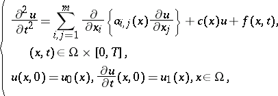 |
with the Dirichlet boundary conditions $u ( x , t ) = 0$ or the Neumann boundary conditions $\sum _ { i ,\, j = 1 } ^ { m } a _ { i ,\, j } ( x ) n _ { i } ( x ) \partial u / \partial x _ { j } = 0$, $( x , t ) \in \partial \Omega \times [ 0 , T ]$.
Here, $\Omega \subset \mathbf{R} ^ { m }$ is a bounded domain with smooth boundary $\partial \Omega$, $a_{i,j} ( x ) = a _ { j , i } ( x )$ and $c ( x ) > 0$ are smooth real functions on $\Omega$ such that $\sum _ { i ,\, j = 1 } ^ { m } a _ { i ,\, j } ( x ) \xi _ { i } \xi _ { j } \geq \delta | \xi | ^ { 2 }$ for all $\xi = ( \xi _ { 1 } , \ldots , \xi _ { m } ) \in \mathbf R ^ { m }$, with some fixed $\delta > 0$; $n = ( n _{1} , \ldots , n _ { m } )$ is the unit outward normal vector to $\partial \Omega$. Also, $f ( x , t )$, $u_{0} ( x )$, $u _ { 1 } ( x )$ are given functions. The function $u ( x , t )$ is the unknown function.
One can state this problem in the abstract form
\begin{equation} \tag{a1} \left\{ \begin{array} { l } { \frac { d ^ { 2 } u } { d t ^ { 2 } } + A u = f ( t ) , \qquad t \in [ 0 , T ], } \\ { u ( 0 ) = u _ { 0 } , \frac { d u } { d t } ( 0 ) = u _ { 1 }, } \end{array} \right. \end{equation}
which is considered in the Hilbert space $L ^ { 2 } ( \Omega )$. Here, $A ( t )$ is the self-adjoint operator of $L ^ { 2 } ( \Omega )$ determined from the symmetric sesquilinear form
\begin{equation} \tag{a2} a ( u , v ) = \int _ { \Omega } \left[ \sum _ { i , j = 1 } ^ { m } a _ { i , j } \frac { \partial u } { \partial x _ { i } } \frac { \partial \bar{v} } { \partial x _ { j } } + c ( x ) u \bar{v} \right] d x \end{equation}
on the space $V$, see [a1], where $V = H _ { 0 } ^ { 1 } ( \Omega )$ (respectively $V = H ^ { 1 } ( \Omega )$) when the boundary conditions are Dirichlet (respectively, Neumann), by the relation $A u = f$ if and only if $a ( u , v ) = ( f , v ) _ { L ^ { 2 }}$ for all $v \in V$. There are several ways to handle this abstract problem.
Let $X$ be a Banach space. A strongly continuous function $S ( t )$ of $t \in \mathbf{R}$ with values in $L ( X )$ is called a cosine function if it satisfies $S ( s + t ) + S ( s - t ) = 2 S ( s ) S ( t )$, $s , t \in \mathbf{R}$, and $S ( 0 ) = 1$. Its infinitesimal generator $A$ is defined by $A = S ^ { \prime \prime } ( 0 )$, with $D ( A ) = \left\{ u \in X : S ( . ) u \in C ^ { 2 } ( \mathbf{R} ; X ) \right\}$. The theory of cosine functions, which is very similar to the theory of semi-groups, was originated by S. Kurera [a2] and was developed by H.O. Fattorini [a3] and others.
A necessary and sufficient condition for a closed linear operator $A$ to be the generator of a cosine family is known. The operator determined by (a2) is easily shown to generate a cosine function which provides a fundamental solution for (a1).
Suppose one sets $v = d u / d t$ in (a1). Then one obtains the equivalent problem
\begin{equation*} \left\{ \begin{array} { l } { \frac { d } { d t } \left( \begin{array} { c } { u } \\ { v } \end{array} \right) + \left( \begin{array} { c c } { 0 } & { - 1 } \\ { A } & { 0 } \end{array} \right) \left( \begin{array} { c } { u } \\ { v } \end{array} \right) = \left( \begin{array} { c } { 0 } \\ { f ( t ) } \end{array} \right) , \quad t \in [ 0 , T ], } \\ { \left( \begin{array} { c } { u ( 0 ) } \\ { v ( 0 ) } \end{array} \right) = \left( \begin{array} { c } { u _ { 0 } } \\ { u _ { 1 } } \end{array} \right), } \end{array} \right. \end{equation*}
which is considered in the product space $V \times L ^ { 2 } ( \Omega )$. Since the equation is of first order, one can apply semi-group theory (see [a4], [a5]). Indeed, the operator
\begin{equation*} \left( \begin{array} { c c } { 0 } & { - 1 } \\ { A } & { 0 } \end{array} \right) \end{equation*}
with its domain $D ( A ) \times V$ is the negative generator of a $C _ { 0 }$ semi-group. The theory of semi-groups of abstract evolution equations provides the existence of a unique solution $u \in C ( [ 0 , T ] ; H ^ { 2 } ( \Omega ) ) \cap C ^ { 2 } ( [ 0 , T ] ; L ^ { 2 } ( \Omega ) )$ of (a1) for $f \in C ( [ 0 , T ] ; V )$ and $u _ { 0 } \in D ( A )$, $u _ { 1 } \in V$.
This method is also available for a non-autonomous equation
\begin{equation} \tag{a3} \frac { d ^ { 2 } u } { d t ^ { 2 } } + A ( t ) u = f ( t ) , t \in [ 0 , T ]. \end{equation}
In the case of Neumann boundary conditions, the difficulty arises that the domain of
\begin{equation*} \left( \begin{array} { c c } { 0 } & { - 1 } \\ { A ( t ) } & { 0 } \end{array} \right) \end{equation*}
may change with $t$. One way to avoid this is to introduce the extension $\mathcal{A} ( t )$ of $A ( t )$ defined by $a ( t ; u , v ) = \langle \mathcal{A} ( t ) u , v \rangle _ { (H^1)^ { \prime } \times H^1}$ for all $v \in H ^ { 1 } ( \Omega )$. Since $\mathcal{A} ( t )$ is a bounded operator from $H ^ { 1 } ( \Omega )$ into $( H ^ { 1 } ( \Omega ) ) ^ { \prime }$, the operator
\begin{equation*} \left( \begin{array} { c c } { 0 } & { - 1 } \\ { {\cal A} ( t ) } & { 0 } \end{array} \right), \end{equation*}
acting in $L ^ { 2 } ( \Omega ) \times ( H ^ { 1 } ( \Omega ) ) ^ { \prime }$, has constant domain.
Another way is to reduce (a3) to
\begin{equation*} \frac { d } { d t } \left( \begin{array} { l } { v _ { 0 } } \\ { v _ { 1 } } \end{array} \right) = \end{equation*}
\begin{equation*} = \left( \begin{array} { c c } { \frac { d A ( t ) ^ { 1 / 2 } } { d t } A ( t ) ^ { - 1 / 2 } } & { i A ( t ) ^ { 1 / 2 } } \\ { i A ( t ) ^ { 1 / 2 } } & { 0 } \end{array} \right) \left( \begin{array} { c } { v _ { 0 } } \\ { v _ { 1 } } \end{array} \right) + \left( \begin{array} { c } { 0 } \\ { f ( t ) } \end{array} \right) ,\, t \in [ 0 , T ], \end{equation*}
by setting $v _ { 0 } = i A ( t ) ^ { 1 / 2 } u$, $v _ { 1 } = d u / d t$, under the assumption that $A ( t ) ^ { 1 / 2 }$ is strongly differentiable with values in $L ( H ^ { 1 } ( \Omega ) , L ^ { 2 } ( \Omega ) )$. Obviously, the linear operator of the coefficient has constant domain $H ^ { 1 } ( \Omega ) \times H ^ { 1 } ( \Omega )$. Differentiability of the square root $A ( t ) ^ { 1 / 2 }$ was studied in [a6], [a7].
In order to consider in (a1) the case when $f \in L ^ { 2 } ( [ 0 , T ] ; L ^ { 2 } ( \Omega ) )$, one has to use the Lions–Magenes variational formulation. In this, one is concerned with the solution $u$ of the problem
\begin{equation*} \left. \begin{cases} { \left( \frac { d ^ { 2 } u } { d t ^ { 2 } } , v \right) _ { L ^ { 2 } } + a ( u , v ) = ( f ( t ) , v ) _ { L ^ { 2 } } }, \\ { \text { a.e. } t \in [ 0 , T ] , v \in V ,} \\ { u ( 0 ) = u _ { 0 } , \frac { d u } { d t } ( 0 ) = u _ { 1 }. } \end{cases} \right. \end{equation*}
The existence of a unique solution $u \in L ^ { 2 } ( [ 0 , T ] ; H ^ { 2 } ( \Omega ) ) \cap H ^ { 2 } ( [ 0 , T ] ; L ^ { 2 } ( \Omega ) )$ has been proved if $f \in H ^ { 1 } ( [ 0 , T ] ; L ^ { 2 } ( \Omega ) )$ and $u _ { 0 } \in D ( A )$, $u _ { 1 } \in V$; see [a8], Chap. 5.
This method is also available for a non-autonomous equation (a3).
The variational method enables one to take $f ( x , t )$ from a wide class, an advantage that is very useful in, e.g., the study of optimal control problems. On the other hand, the semi-group method provides regular solutions, which is often important in applications to non-linear problems. Using these approaches, many papers have been devoted to non-linear wave equations.
References
| [a1] | J.-L. Lions, "Espaces d'interpolation et domaines de puissances fractionnaires d'opérateurs" J. Math. Soc. Japan , 14 (1962) pp. 233–241 |
| [a2] | S. Kurepa, "A cosine functional equation in Hilbert spaces" Canad. J. Math. , 12 (1960) pp. 45–50 |
| [a3] | H.O. Fattorini, "Ordinary differential equations in linear topological spaces II" J. Diff. Eq. , 6 (1969) pp. 50–70 |
| [a4] | E. Hille, R.S. Phillips, "Functional analysis and semi-groups" , Amer. Math. Soc. (1957) |
| [a5] | K. Yoshida, "Functional analysis" , Springer (1957) |
| [a6] | A. McIntosh, "Square roots of elliptic operators" J. Funct. Anal. , 61 (1985) pp. 307–327 |
| [a7] | A. Yagi, "Applications of the purely imaginary powers of operators in Hilbert spaces" J. Funct. Anal. , 73 (1987) pp. 216–231 |
| [a8] | J.-L. Lions, E. Magenes, "Problèmes aux limites non homogènes et applications" , 1–2 , Dunod (1968) |
Abstract wave equation. Encyclopedia of Mathematics. URL: http://encyclopediaofmath.org/index.php?title=Abstract_wave_equation&oldid=17290