Viscous fingering

An interface between two fluids presents a resistance towards an increase of its surface area. This interface has a surface tension which opposes such an increase. This is the property giving a liquid drop its spherical shape: A sphere has a minimal surface for a given volume of fluid. T. Young and P.S. Laplace rationalized this scenario by postulating the Young–Laplace law.

In viscous fingering, where a less viscous fluid, such as air, pushes a more viscous fluid, such as an oil, in thin rectangular cells (known as Hele-Shaw cells), surface tension plays an important role in determining the shape and properties of the fingers. The basic experimental situation to obtain viscous fingers is as follows (here, the focus is on the linear channel geometry, but such experiments can also be obtained in circular cells). One usually uses two thick glass plates and a thin plastic sheet to obtain a linear Hele-Shaw cell [a8]. The plastic sheet serves as a spacer between the glass plates once they are brought into contact with each other. A long rectangular canal can be cut in the middle of the plastic sheet, which is then sandwiched between the glass plates to obtain a thin linear rectangular channel. The thickness of this canal is fixed by the thickness of the plastic sheet. Through holes drilled in the upper glass plates one then injects the viscous fluid to fill up the cell. Subsequently, air is injected at constant pressure or constant flux to push the oil out of this canal (see Fig.a2 for a scheme of the cell). The interface between the air and the oil is then unstable: the flat interface takes a curved shape. This instability is well known and from the pioneering work of P.G. Saffman and G.I. Taylor in the 1950s [a7], it is known that the finger of air has a width which decreases with the velocity of the finger. The most mysterious aspect observed by Saffman and Taylor is that the limiting width of the fingers obtained at high velocities is very close to half the channel width. This property was not explained until the 1980s, although Saffman and Taylor did calculate the shape of the finger they obtained in their experiments.

Figure: v130070a

A Saffman–Taylor finger obtained with air injected in a viscous fluid. This finger has a width very close to half the channel width. The gray region delimiting the finger contains the fluid, while the white region contains air. The black dots represent the shape obtained from the Saffman–Taylor solution

Figure: v130070b

Scheme of the linear Hele-Shaw cell: two thick glass plates with two tubes attached to inject the less viscous fluid and to recover the fluid being pushed. The gray part is the plastic sheet of thickness into which a linear channel of width is cut

See below for the basic equations governing this problem and some hints as to how it was resolved using techniques from complex analysis and perturbation theory in the 1980s. See [a11], [a6], [a3] for accessible reviews of the experiment and phenomena.

The use of a Hele-Shaw cell permits one to use a simplified version of the equations governing the flow of the fluids. Basically, the Navier–Stokes equations are simplified to keep just the pressure gradient term and the dissipative term. This approximation is known as Darcy's law and is obeyed by flows in porous media, for example. In a sense, the linear Hele-Shaw cell is a simple porous medium, as was shown by H.J.S. Hele-Shaw [a8]. This equation is written as follows:

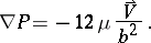Here, the gradient is in the plane of the cell, denoted by (the finger propagates along the direction with being the transverse direction), is the pressure, is the fluid shear viscosity, is the velocity of the fluid in the -plane far from the fingertip and averaged over the vertical gap of thickness ( being the spacing between the plates fixed by the thickness of the plastic sheet). One can rewrite this equation in terms of a velocity potential such that ; due to the incompressibility of the fluid this potential obeys the Laplace equation . Suppose the following boundary conditions on the interface apply:

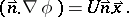Here, is the normal to the interface delimiting the finger, is the unit vector in the direction of propagation of the finger and is the velocity of the tip. The finger is supposed to advance at constant velocity and keeps a constant width , where is the width of the channel and is the relative width of the finger [a7]. The potential at the interface is

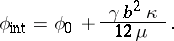Here, is the surface tension of the interface and is the curvature of the interface. The additional term in the potential expresses the effect of surface tension due to the Young–Laplace law. is the potential inside the less viscous fluid (which can be taken as inviscid without loss of generality). It is clear that far behind the fingertip the potential is zero while far ahead of the fingertip the viscous fluid is moving with velocity . The problem is now to determine the relation between the coordinates of the interface and . In 1980, J.W. McLean and P.G. Saffman [a5] suggested a way of rewriting the equations in complex representation which came in handy for later work. One writes the coordinates in the complex plane as and (where is the stream function). The transformation is a conformal mapping from the flow region delimited by the finger and the walls of the channel into an infinite strip of unit width in the potential plane. The conformal mapping maps the flow region into the upper -plane. This transforms the interface between the tails and the tip of the finger into the real segment . The boundary corresponds to the tail of the finger, for which , and corresponds to the tip, for which . The problem now reduces to finding in terms of . However, it turns out to be simpler to study the quantity ; it is the complex velocity and may be written as , since the velocity is tangent to the interface (with the angle between and the tangent to the interface). The modulus at the interface can be written as , where measures arclength along the interface starting from the tip. By invoking the analytic properties of , the following relation can be established between and :

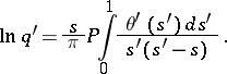Besides this relation there is a second one, dictated by the Young–Laplace law:

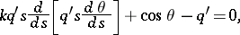where

These two equations are to be solved with the following boundary conditions:

at the tail of the finger: and ;

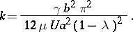
at the tip of the finger: and . If a solution of these equations is found, the value of (which is the quantity that needs to be determined) as well as its dependence on physical parameters, such as the velocity of the finger, the viscosity of the fluid and especially the surface tension, can be found from the relation:

At this point the equations are complete. Of course, the difficulty is in solving these equations. For the case of zero surface tension (), one finds a continuum of solutions for the finger shape, parametrized by the value of which remains unknown. The family of solutions first found by Saffman and Taylor is written as:

with . In the coordinates and , this solution for the interface shape reads:

The problem now is to find a selection mechanism for the allowed values of . This problem was not resolved until 1986, when three different groups [a9], [a10], [a1], [a2] studied the small- limit of these equations using techniques from perturbation theory and showed that the continuum of solutions breaks into a discrete set of solutions with the value of decreasing to its well-known value of as approaches . This calculation is rather involved; see [a9], [a10], [a1], [a2].

The use of complex fluids such as, e.g., gels, clays, polymeric solutions, mixtures of water and surfactants can give rise to new morphologies of the interfaces in Hele-Shaw cells [a6].

In the above, the viscosity of the fluid as well as the surface tension of the interface were considered to be constant. For complicated fluids these physical quantities may depend on the velocity of the fluid and therefore become variable. This complicates the mathematical analysis of the instability; however, some progress has been made [a4].

References

[a1]	B.I. Shraiman, Phys. Rev. Lett. , 56 (1986) pp. 2028
[a2]	D.C. Hong, J. Langer, Phys. Rev. Lett. , 56 (1986) pp. 2032
[a3]	D. Bensimon, L.P. Kadanoff, S. Liang, B.I. Shraiman, C. Tang, Rev. Mod. Phys. , 58 (1986) pp. 977
[a4]	D. Bonn, H. Kellay, J. Meunier, Philos. Mag. B , 78 (1998) pp. 131–142
[a5]	J.W. McLean, P.G. Saffman, J. Fluid Mech. , 102 (1981) pp. 455
[a6]	K.V. McCloud, J.V. Maher, Phys. Rept. , 260 (1995) pp. 139
[a7]	P.G. Saffman, G.I. Taylor, Proc. Royal Soc. London A , 245 (1958) pp. 312
[a8]	H.J.S. Hele-Shaw, Nature , 58 (1898) pp. 34
[a9]	R. Combescot, T. Dombre, V. Hakim, Y. Pomeau, A. Pumir, Phys. Rev. Lett. , 56 (1986) pp. 2036
[a10]	R. Combescot, T. Dombre, V. Hakim, Y. Pomeau, A. Pumir, Phys. Rev. A , 37 (1988) pp. 1270
[a11]	P. Pelcé, A. Libchaber, "Dynamics of curved fronts" , Perspectives in Physics , Acad. Press (1997)