|
|
| (9 intermediate revisions by 3 users not shown) |
| Line 1: |
Line 1: |
| − | ''B-series''
| + | <!-- |
| | + | b1110701.png |
| | + | $#A+1 = 106 n = 0 |
| | + | $#C+1 = 106 : ~/encyclopedia/old_files/data/B111/B.1101070 Butcher series, |
| | + | Automatically converted into TeX, above some diagnostics. |
| | + | Please remove this comment and the {{TEX|auto}} line below, |
| | + | if TeX found to be correct. |
| | + | --> |
| | | | |
| − | Let <img align="absmiddle" border="0" src="https://www.encyclopediaofmath.org/legacyimages/b/b111/b111070/b1110701.png" /> be an [[Analytic function|analytic function]] satisfying an ordinary differential equation <img align="absmiddle" border="0" src="https://www.encyclopediaofmath.org/legacyimages/b/b111/b111070/b1110702.png" />. A Butcher series for <img align="absmiddle" border="0" src="https://www.encyclopediaofmath.org/legacyimages/b/b111/b111070/b1110703.png" /> is a series of the form
| + | {{TEX|auto}} |
| | + | {{TEX|done}} |
| | | | |
| − | <table class="eq" style="width:100%;"> <tr><td valign="top" style="width:94%;text-align:center;"><img align="absmiddle" border="0" src="https://www.encyclopediaofmath.org/legacyimages/b/b111/b111070/b1110704.png" /></td> </tr></table>
| + | ''B-series'' |
| | | | |
| − | where <img align="absmiddle" border="0" src="https://www.encyclopediaofmath.org/legacyimages/b/b111/b111070/b1110705.png" /> is the set of rooted trees, <img align="absmiddle" border="0" src="https://www.encyclopediaofmath.org/legacyimages/b/b111/b111070/b1110706.png" /> is the coefficient for the series associated with the tree <img align="absmiddle" border="0" src="https://www.encyclopediaofmath.org/legacyimages/b/b111/b111070/b1110707.png" />, <img align="absmiddle" border="0" src="https://www.encyclopediaofmath.org/legacyimages/b/b111/b111070/b1110708.png" /> is the elementary differential associated with the tree <img align="absmiddle" border="0" src="https://www.encyclopediaofmath.org/legacyimages/b/b111/b111070/b1110709.png" />, <img align="absmiddle" border="0" src="https://www.encyclopediaofmath.org/legacyimages/b/b111/b111070/b11107010.png" /> is a stepsize or <img align="absmiddle" border="0" src="https://www.encyclopediaofmath.org/legacyimages/b/b111/b111070/b11107011.png" />-increment, and <img align="absmiddle" border="0" src="https://www.encyclopediaofmath.org/legacyimages/b/b111/b111070/b11107012.png" />, often called the order of the tree <img align="absmiddle" border="0" src="https://www.encyclopediaofmath.org/legacyimages/b/b111/b111070/b11107013.png" />, is the number of nodes in the tree <img align="absmiddle" border="0" src="https://www.encyclopediaofmath.org/legacyimages/b/b111/b111070/b11107014.png" />. All terms will be defined below. For a more thorough discussion of Butcher series, see [[#References|[a1]]] or [[#References|[a2]]].
| + | Let $ y : \mathbf R \rightarrow {\mathbf R ^ {d} } $ |
| | + | be an [[Analytic function|analytic function]] satisfying an ordinary differential equation $ y ^ \prime ( x ) = f ( y ( x ) ) $. |
| | + | A Butcher series for $ y $ |
| | + | is a series of the form |
| | | | |
| − | ==Definitions.==
| + | $$ |
| − | A tree is a connected acyclic graph (cf. also [[Graph|Graph]]). A rooted tree is a tree with a distinguished node, called the root (which is drawn at the bottom of the sample trees in the Table). Two rooted trees <img align="absmiddle" border="0" src="https://www.encyclopediaofmath.org/legacyimages/b/b111/b111070/b11107015.png" /> and <img align="absmiddle" border="0" src="https://www.encyclopediaofmath.org/legacyimages/b/b111/b111070/b11107016.png" /> are isomorphic (i.e., equivalent) if and only if there is a [[Bijection|bijection]] <img align="absmiddle" border="0" src="https://www.encyclopediaofmath.org/legacyimages/b/b111/b111070/b11107017.png" /> from the nodes of <img align="absmiddle" border="0" src="https://www.encyclopediaofmath.org/legacyimages/b/b111/b111070/b11107018.png" /> to the nodes of <img align="absmiddle" border="0" src="https://www.encyclopediaofmath.org/legacyimages/b/b111/b111070/b11107019.png" /> such that <img align="absmiddle" border="0" src="https://www.encyclopediaofmath.org/legacyimages/b/b111/b111070/b11107020.png" /> maps the root of <img align="absmiddle" border="0" src="https://www.encyclopediaofmath.org/legacyimages/b/b111/b111070/b11107021.png" /> to the root of <img align="absmiddle" border="0" src="https://www.encyclopediaofmath.org/legacyimages/b/b111/b111070/b11107022.png" /> and any two nodes <img align="absmiddle" border="0" src="https://www.encyclopediaofmath.org/legacyimages/b/b111/b111070/b11107023.png" /> and <img align="absmiddle" border="0" src="https://www.encyclopediaofmath.org/legacyimages/b/b111/b111070/b11107024.png" /> are connected by an edge in <img align="absmiddle" border="0" src="https://www.encyclopediaofmath.org/legacyimages/b/b111/b111070/b11107025.png" /> if and only if <img align="absmiddle" border="0" src="https://www.encyclopediaofmath.org/legacyimages/b/b111/b111070/b11107026.png" /> and <img align="absmiddle" border="0" src="https://www.encyclopediaofmath.org/legacyimages/b/b111/b111070/b11107027.png" /> are connected by an edge in <img align="absmiddle" border="0" src="https://www.encyclopediaofmath.org/legacyimages/b/b111/b111070/b11107028.png" />.
| + | B ( a,y ( x ) ) = \sum _ {t \in T } a ( t ) F ( t ) ( y ( x ) ) { |
| | + | \frac{h ^ {\rho ( t ) } }{\rho ( t ) ! } |
| | + | } , |
| | + | $$ |
| | | | |
| − | The following bracket notation for rooted trees is very useful. Let <img align="absmiddle" border="0" src="https://www.encyclopediaofmath.org/legacyimages/b/b111/b111070/b11107029.png" /> and <img align="absmiddle" border="0" src="https://www.encyclopediaofmath.org/legacyimages/b/b111/b111070/b11107030.png" /> be the trees with zero and one node, respectively. For rooted trees <img align="absmiddle" border="0" src="https://www.encyclopediaofmath.org/legacyimages/b/b111/b111070/b11107031.png" /> with <img align="absmiddle" border="0" src="https://www.encyclopediaofmath.org/legacyimages/b/b111/b111070/b11107032.png" /> for <img align="absmiddle" border="0" src="https://www.encyclopediaofmath.org/legacyimages/b/b111/b111070/b11107033.png" />, let <img align="absmiddle" border="0" src="https://www.encyclopediaofmath.org/legacyimages/b/b111/b111070/b11107034.png" /> be the rooted tree formed by connecting a new root to the roots of each of <img align="absmiddle" border="0" src="https://www.encyclopediaofmath.org/legacyimages/b/b111/b111070/b11107035.png" />. Clearly, <img align="absmiddle" border="0" src="https://www.encyclopediaofmath.org/legacyimages/b/b111/b111070/b11107036.png" /> and any rooted tree formed by permuting the subtrees <img align="absmiddle" border="0" src="https://www.encyclopediaofmath.org/legacyimages/b/b111/b111070/b11107037.png" /> of <img align="absmiddle" border="0" src="https://www.encyclopediaofmath.org/legacyimages/b/b111/b111070/b11107038.png" /> is isomorphic to <img align="absmiddle" border="0" src="https://www.encyclopediaofmath.org/legacyimages/b/b111/b111070/b11107039.png" />. The rooted trees with at most four nodes are displayed in the table below.''''''<table border="0" cellpadding="0" cellspacing="0" style="background-color:black;"> <tr><td> <table border="0" cellspacing="1" cellpadding="4" style="background-color:black;"> <tbody> <tr> <td colname="1" style="background-color:white;" colspan="1"><img align="absmiddle" border="0" src="https://www.encyclopediaofmath.org/legacyimages/b/b111/b111070/b11107040.png" /></td> <td colname="2" style="background-color:white;" colspan="1"><img align="absmiddle" border="0" src="https://www.encyclopediaofmath.org/legacyimages/b/b111/b111070/b11107041.png" /></td> </tr> <tr> <td colname="1" style="background-color:white;" colspan="1"><img align="absmiddle" border="0" src="https://www.encyclopediaofmath.org/legacyimages/b/b111/b111070/b11107042.png" /></td> <td colname="2" style="background-color:white;" colspan="1">
| + | where $ T $ |
| | + | is the set of [[rooted tree]]s, $ a ( t ) \in \mathbf R $ |
| | + | is the coefficient for the series associated with the tree $ t $, |
| | + | $ F ( t ) ( y ( x ) ) \in \mathbf R ^ {d} $ |
| | + | is the elementary differential associated with the tree $ t $, |
| | + | $ h \in \mathbf R $ |
| | + | is a stepsize or $ x $- |
| | + | increment, and $ \rho ( t ) $, |
| | + | often called the order of the tree $ t $, |
| | + | is the number of nodes in the tree $ t $. |
| | + | All terms will be defined below. For a more thorough discussion of Butcher series, see [[#References|[a1]]] or [[#References|[a2]]]. |
| | | | |
| − | <img style="border:1px solid;" src="https://www.encyclopediaofmath.org/legacyimages/common_img/" />
| + | ==Definitions== |
| | + | A tree is a connected acyclic graph (cf. also [[Graph|Graph]]). A rooted tree is a tree with a distinguished node, called the root (which is drawn at the bottom of the sample trees in the Table). Two rooted trees $t$ |
| | + | and $\widehat{t}$ |
| | + | are isomorphic (''i.e.'' equivalent) if and only if there is a [[Bijection|bijection]] $\sigma $ |
| | + | from the nodes of $t$ to the nodes of $\widehat{t}$ |
| | + | such that $ \sigma $ maps the root of $ t $ |
| | + | to the root of $ {\widehat{t} } $ |
| | + | and any two nodes $ n _ {1} $ |
| | + | and $ n _ {2} $ are connected by an edge in $ t $ |
| | + | if and only if $ \sigma ( n _ {1} ) $ |
| | + | and $ \sigma ( n _ {2} ) $ |
| | + | are connected by an edge in $ {\widehat{t} } $. |
| | | | |
| − | </td> </tr> <tr> <td colname="1" style="background-color:white;" colspan="1"><img align="absmiddle" border="0" src="https://www.encyclopediaofmath.org/legacyimages/b/b111/b111070/b11107043.png" /></td> <td colname="2" style="background-color:white;" colspan="1">
| + | The following bracket notation for rooted trees is very useful. Let $\bullet$ |
| | + | be the tree with one node. For rooted trees $ t_{1} \dots t _ {m} $ |
| | + | with $ \rho ( t _ {i} ) \geq 1 $ |
| | + | for $ i = 1 \dots m $, |
| | + | let $ t = [ t _ {1} \dots t _ {m} ] $ |
| | + | be the rooted tree formed by connecting a new root to the roots of each of $ t _ {1} \dots t _ {m} $. |
| | + | Clearly, $ \rho ( t ) = 1 + \sum _ {i = 1 } ^ {m} \rho ( t _ {i} ) $ |
| | + | and any rooted tree formed by permuting the subtrees $ t _ {1} \dots t _ {m} $ |
| | + | of $ t $ |
| | + | is isomorphic to $ t $. |
| | | | |
| − | <img style="border:1px solid;" src="https://www.encyclopediaofmath.org/legacyimages/common_img/" />
| + | The rooted trees with at most four nodes are displayed in the table below. |
| | | | |
| − | </td> </tr> <tr> <td colname="1" style="background-color:white;" colspan="1"><img align="absmiddle" border="0" src="https://www.encyclopediaofmath.org/legacyimages/b/b111/b111070/b11107044.png" /></td> <td colname="2" style="background-color:white;" colspan="1">
| + | {| class="wikitable" |
| | + | |- |
| | + | | $t_1$ || $t_2=[t_1]$ || $ t_{3} = [t_{1},t_{1}]$ || $t_4 = [t_2]$ |
| | + | |- |
| | + | | [[File:Rooted tree 0.svg|50px]] || [[File:Rooted tree 10.svg|50px]] || [[File:Rooted tree 200.svg|100px]]|| [[File:Rooted tree 110.svg|50px]] |
| | + | |- |
| | + | |} |
| | | | |
| − | <img style="border:1px solid;" src="https://www.encyclopediaofmath.org/legacyimages/common_img/" />
| + | {| class="wikitable" |
| | + | |- |
| | + | | $t_5 =[t_1,t_1,t_1]$ || $t_6=[t_2,t_1]$ || $ t_{7} = [t_{3}]$ || $ t_{8} = [t_4]$ |
| | + | |- |
| | + | | [[File:Rooted tree 3000.svg|100px]] || [[File:Rooted tree 2100.svg|100px]] || [[File:Rooted tree 1200.svg|100px]]|| [[File:Rooted tree 1110.svg|50px]] |
| | + | |- |
| | + | |} |
| | | | |
| − | </td> </tr> <tr> <td colname="1" style="background-color:white;" colspan="1"><img align="absmiddle" border="0" src="https://www.encyclopediaofmath.org/legacyimages/b/b111/b111070/b11107045.png" /></td> <td colname="2" style="background-color:white;" colspan="1">
| + | Using this bracket notation for rooted trees, one can recursively define elementary differentials, as follows. Let |
| − | | |
| − | <img style="border:1px solid;" src="https://www.encyclopediaofmath.org/legacyimages/common_img/" />
| |
| − | | |
| − | </td> </tr> <tr> <td colname="1" style="background-color:white;" colspan="1"><img align="absmiddle" border="0" src="https://www.encyclopediaofmath.org/legacyimages/b/b111/b111070/b11107046.png" /></td> <td colname="2" style="background-color:white;" colspan="1">
| |
| − | | |
| − | <img style="border:1px solid;" src="https://www.encyclopediaofmath.org/legacyimages/common_img/" />
| |
| | | | |
| − | </td> </tr> <tr> <td colname="1" style="background-color:white;" colspan="1"><img align="absmiddle" border="0" src="https://www.encyclopediaofmath.org/legacyimages/b/b111/b111070/b11107047.png" /></td> <td colname="2" style="background-color:white;" colspan="1">
| + | $$ |
| | + | F ( \emptyset ) ( y ( x ) ) = y ( x ) , \quad F ( \bullet ) ( y ( x ) ) = f ( y ( x ) ) , |
| | + | $$ |
| | | | |
| − | <img style="border:1px solid;" src="https://www.encyclopediaofmath.org/legacyimages/common_img/" />
| + | and, for $ t = [ t _ {1} \dots t _ {m} ] $ |
| | + | with $ \rho ( t _ {i} ) \geq 1 $ |
| | + | for $ i = 1 \dots m $, |
| | | | |
| − | </td> </tr> <tr> <td colname="1" style="background-color:white;" colspan="1"><img align="absmiddle" border="0" src="https://www.encyclopediaofmath.org/legacyimages/b/b111/b111070/b11107048.png" /></td> <td colname="2" style="background-color:white;" colspan="1">
| + | $$ |
| | + | F ( t ) ( y ( x ) ) = |
| | + | $$ |
| | | | |
| − | <img style="border:1px solid;" src="https://www.encyclopediaofmath.org/legacyimages/common_img/" />
| + | $$ |
| | + | = |
| | + | f ^ {( m ) } ( y ( x ) ) ( F ( t _ {1} ) ( y ( x ) ) \dots F ( t _ {m} ) ( y ( x ) ) ) , |
| | + | $$ |
| | | | |
| − | </td> </tr> <tr> <td colname="1" style="background-color:white;" colspan="1"><img align="absmiddle" border="0" src="https://www.encyclopediaofmath.org/legacyimages/b/b111/b111070/b11107049.png" /></td> <td colname="2" style="background-color:white;" colspan="1">
| + | where $ f ^ {( m ) } ( y ( x ) ) $, |
| | + | the $ m $ |
| | + | th derivative of $ f $ |
| | + | with respect to $ y $, |
| | + | is a multi-linear mapping. |
| | | | |
| − | <img style="border:1px solid;" src="https://www.encyclopediaofmath.org/legacyimages/common_img/" />
| + | Since $ y ( x ) $ |
| − | | + | satisfies $ y ^ \prime ( x ) = f ( y ( x ) ) $, |
| − | </td> </tr> </tbody> </table>
| + | it is not hard to show that |
| − | | |
| − | </td></tr> </table>
| |
| − | | |
| − | Using this bracket notation for rooted trees, one can recursively define elementary differentials, as follows. Let
| |
| | | | |
| − | <table class="eq" style="width:100%;"> <tr><td valign="top" style="width:94%;text-align:center;"><img align="absmiddle" border="0" src="https://www.encyclopediaofmath.org/legacyimages/b/b111/b111070/b11107050.png" /></td> </tr></table>
| + | $$ |
| | + | y ^ {( i ) } ( x ) = \sum _ {t \in T _ {i} } \alpha ( t ) F ( t ) ( y ( x ) ) , |
| | + | $$ |
| | | | |
| − | and, for <img align="absmiddle" border="0" src="https://www.encyclopediaofmath.org/legacyimages/b/b111/b111070/b11107051.png" /> with <img align="absmiddle" border="0" src="https://www.encyclopediaofmath.org/legacyimages/b/b111/b111070/b11107052.png" /> for <img align="absmiddle" border="0" src="https://www.encyclopediaofmath.org/legacyimages/b/b111/b111070/b11107053.png" />,
| + | where $ y ^ {( i ) } ( x ) $ |
| | + | is the $ i $ |
| | + | th derivative of $ y $ |
| | + | with respect to $ x $, |
| | + | $ T _ {i} = \{ {t \in T } : {\rho ( t ) = i } \} $, |
| | + | and $ \alpha ( t ) $ |
| | + | is the number of distinct ways of labeling the nodes of $ t $ |
| | + | with the integers $ \{ 1 \dots \rho ( t ) \} $ |
| | + | such that the labels increase as you follow any path from the root to a leaf of $ t $. |
| | + | Consequently, one can write the [[Taylor series|Taylor series]] for $ y ( x ) $ |
| | + | as a Butcher series: |
| | | | |
| − | <table class="eq" style="width:100%;"> <tr><td valign="top" style="width:94%;text-align:center;"><img align="absmiddle" border="0" src="https://www.encyclopediaofmath.org/legacyimages/b/b111/b111070/b11107054.png" /></td> </tr></table>
| + | \begin{equation} |
| | + | \label{eq:1} |
| | + | y ( x + h ) = \sum _ {i = 0 } ^ \infty y ^ {( i ) } ( x ) { |
| | + | \frac{h ^ {i} }{i! } |
| | + | } = |
| | + | \end{equation} |
| | | | |
| − | <table class="eq" style="width:100%;"> <tr><td valign="top" style="width:94%;text-align:center;"><img align="absmiddle" border="0" src="https://www.encyclopediaofmath.org/legacyimages/b/b111/b111070/b11107055.png" /></td> </tr></table>
| + | $$ |
| | + | = |
| | + | \sum _ {t \in T } \alpha ( t ) F ( t ) ( y ( x ) ) { |
| | + | \frac{h ^ {\rho ( t ) } }{\rho ( t ) ! } |
| | + | } . |
| | + | $$ |
| | | | |
| − | where <img align="absmiddle" border="0" src="https://www.encyclopediaofmath.org/legacyimages/b/b111/b111070/b11107056.png" />, the <img align="absmiddle" border="0" src="https://www.encyclopediaofmath.org/legacyimages/b/b111/b111070/b11107057.png" />th derivative of <img align="absmiddle" border="0" src="https://www.encyclopediaofmath.org/legacyimages/b/b111/b111070/b11107058.png" /> with respect to <img align="absmiddle" border="0" src="https://www.encyclopediaofmath.org/legacyimages/b/b111/b111070/b11107059.png" />, is a multi-linear mapping.
| + | The importance of Butcher series stems from their use to derive and to analyze numerical methods for differential equations. For example, consider the $ s $- |
| | + | stage Runge–Kutta formula (cf. [[Runge–Kutta method|Runge–Kutta method]]) |
| | | | |
| − | Since <img align="absmiddle" border="0" src="https://www.encyclopediaofmath.org/legacyimages/b/b111/b111070/b11107060.png" /> satisfies <img align="absmiddle" border="0" src="https://www.encyclopediaofmath.org/legacyimages/b/b111/b111070/b11107061.png" />, it is not hard to show that
| + | \begin{equation}\label{eq:2} |
| | + | y _ {n + 1 } = y _ {n} + h \sum _ {i = 1 } ^ { s } b _ {i} k _ {i} , |
| | + | \end{equation} |
| | | | |
| − | <table class="eq" style="width:100%;"> <tr><td valign="top" style="width:94%;text-align:center;"><img align="absmiddle" border="0" src="https://www.encyclopediaofmath.org/legacyimages/b/b111/b111070/b11107062.png" /></td> </tr></table>
| + | $$ |
| | + | k _ {i} = f \left ( y _ {n} + h \sum _ {j = 1 } ^ { s } a _ {ij } k _ {j} \right ) , |
| | + | $$ |
| | | | |
| − | where <img align="absmiddle" border="0" src="https://www.encyclopediaofmath.org/legacyimages/b/b111/b111070/b11107063.png" /> is the <img align="absmiddle" border="0" src="https://www.encyclopediaofmath.org/legacyimages/b/b111/b111070/b11107064.png" />th derivative of <img align="absmiddle" border="0" src="https://www.encyclopediaofmath.org/legacyimages/b/b111/b111070/b11107065.png" /> with respect to <img align="absmiddle" border="0" src="https://www.encyclopediaofmath.org/legacyimages/b/b111/b111070/b11107066.png" />, <img align="absmiddle" border="0" src="https://www.encyclopediaofmath.org/legacyimages/b/b111/b111070/b11107067.png" />, and <img align="absmiddle" border="0" src="https://www.encyclopediaofmath.org/legacyimages/b/b111/b111070/b11107068.png" /> is the number of distinct ways of labeling the nodes of <img align="absmiddle" border="0" src="https://www.encyclopediaofmath.org/legacyimages/b/b111/b111070/b11107069.png" /> with the integers <img align="absmiddle" border="0" src="https://www.encyclopediaofmath.org/legacyimages/b/b111/b111070/b11107070.png" /> such that the labels increase as you follow any path from the root to a leaf of <img align="absmiddle" border="0" src="https://www.encyclopediaofmath.org/legacyimages/b/b111/b111070/b11107071.png" />. Consequently, one can write the [[Taylor series|Taylor series]] for <img align="absmiddle" border="0" src="https://www.encyclopediaofmath.org/legacyimages/b/b111/b111070/b11107072.png" /> as a Butcher series:
| + | for the ordinary differential equation $ y ^ \prime ( x ) = f ( y ( x ) ) $. |
| | + | Let $ b = ( b _ {1} \dots b _ {s} ) ^ {T} \in \mathbf R ^ {s} $ |
| | + | be the vector of weights and $ A = [ a _ {ij } ] \in \mathbf R ^ {s \times s } $ |
| | + | the coefficient matrix for (a2). Then it can be shown that $ y _ {n + 1 } $ |
| | + | can be written as the Butcher series |
| | | | |
| − | <table class="eq" style="width:100%;"> <tr><td valign="top" style="width:94%;text-align:center;"><img align="absmiddle" border="0" src="https://www.encyclopediaofmath.org/legacyimages/b/b111/b111070/b11107073.png" /></td> <td valign="top" style="width:5%;text-align:right;">(a1)</td></tr></table>
| + | \begin{equation}\label{eq:3} |
| | + | y _ {n + 1 } = \sum _ {t \in T } \alpha ( t ) \psi ( t ) F ( t ) ( y _ {n} ) { |
| | + | \frac{h ^ {\rho ( t ) } }{\rho ( t ) ! } |
| | + | } , |
| | + | \end{equation} |
| | | | |
| − | <table class="eq" style="width:100%;"> <tr><td valign="top" style="width:94%;text-align:center;"><img align="absmiddle" border="0" src="https://www.encyclopediaofmath.org/legacyimages/b/b111/b111070/b11107074.png" /></td> </tr></table>
| + | where the coefficients $ \psi(t) \in \mathbf R $, |
| | + | defined below, depend only on the rooted tree $t$ |
| | + | and the coefficients of the formula \eqref{eq:2}. |
| | | | |
| − | The importance of Butcher series stems from their use to derive and to analyze numerical methods for differential equations. For example, consider the <img align="absmiddle" border="0" src="https://www.encyclopediaofmath.org/legacyimages/b/b111/b111070/b11107076.png" />-stage Runge–Kutta formula (cf. [[Runge–Kutta method|Runge–Kutta method]])
| + | To define $ \psi ( t ) $, |
| | + | first let |
| | | | |
| − | <table class="eq" style="width:100%;"> <tr><td valign="top" style="width:94%;text-align:center;"><img align="absmiddle" border="0" src="https://www.encyclopediaofmath.org/legacyimages/b/b111/b111070/b11107077.png" /></td> <td valign="top" style="width:5%;text-align:right;">(a2)</td></tr></table>
| + | $$ |
| | + | \phi ( \emptyset ) = ( 1 \dots 1 ) ^ {T} \in \mathbf R ^ {s} , |
| | + | $$ |
| | | | |
| − | <table class="eq" style="width:100%;"> <tr><td valign="top" style="width:94%;text-align:center;"><img align="absmiddle" border="0" src="https://www.encyclopediaofmath.org/legacyimages/b/b111/b111070/b11107078.png" /></td> </tr></table>
| + | $$ |
| | + | \phi ( \bullet ) = A \phi ( \emptyset ) , |
| | + | $$ |
| | | | |
| − | for the ordinary differential equation <img align="absmiddle" border="0" src="https://www.encyclopediaofmath.org/legacyimages/b/b111/b111070/b11107079.png" />. Let <img align="absmiddle" border="0" src="https://www.encyclopediaofmath.org/legacyimages/b/b111/b111070/b11107080.png" /> be the vector of weights and <img align="absmiddle" border="0" src="https://www.encyclopediaofmath.org/legacyimages/b/b111/b111070/b11107081.png" /> the coefficient matrix for (a2). Then it can be shown that <img align="absmiddle" border="0" src="https://www.encyclopediaofmath.org/legacyimages/b/b111/b111070/b11107082.png" /> can be written as the Butcher series | + | and then, for $ t = [ t _ {1} \dots t _ {m} ] $ |
| | + | with $ \rho ( t _ {i} ) \geq 1 $ |
| | + | for $ i = 1 \dots m $, |
| | + | define $ \phi ( t ) $ |
| | + | recursively by |
| | | | |
| − | <table class="eq" style="width:100%;"> <tr><td valign="top" style="width:94%;text-align:center;"><img align="absmiddle" border="0" src="https://www.encyclopediaofmath.org/legacyimages/b/b111/b111070/b11107083.png" /></td> <td valign="top" style="width:5%;text-align:right;">(a3)</td></tr></table>
| + | $$ |
| | + | \phi ( t ) = \rho ( t ) A ( \phi ( t _ {1} ) \dots \phi ( t _ {m} ) ) , |
| | + | $$ |
| | | | |
| − | where the coefficients <img align="absmiddle" border="0" src="https://www.encyclopediaofmath.org/legacyimages/b/b111/b111070/b11107084.png" />, defined below, depend only on the rooted tree <img align="absmiddle" border="0" src="https://www.encyclopediaofmath.org/legacyimages/b/b111/b111070/b11107085.png" /> and the coefficients of the formula (a2). | + | where the product of $ \phi $'s in the bracket is taken component-wise. Then |
| | | | |
| − | To define <img align="absmiddle" border="0" src="https://www.encyclopediaofmath.org/legacyimages/b/b111/b111070/b11107086.png" />, first let
| + | $$ |
| | + | \psi ( \emptyset ) = 1, |
| | + | $$ |
| | | | |
| − | <table class="eq" style="width:100%;"> <tr><td valign="top" style="width:94%;text-align:center;"><img align="absmiddle" border="0" src="https://www.encyclopediaofmath.org/legacyimages/b/b111/b111070/b11107087.png" /></td> </tr></table>
| + | $$ |
| | + | \psi ( \bullet ) = \sum _ {i = 1 } ^ { s } b _ {i} , |
| | + | $$ |
| | | | |
| − | <table class="eq" style="width:100%;"> <tr><td valign="top" style="width:94%;text-align:center;"><img align="absmiddle" border="0" src="https://www.encyclopediaofmath.org/legacyimages/b/b111/b111070/b11107088.png" /></td> </tr></table>
| + | and, for $ t = [ t _ {1} \dots t _ {m} ] $ |
| | + | with $ \rho ( t _ {i} ) \geq 1 $ |
| | + | for $ i = 1 \dots m $, |
| | | | |
| − | and then, for <img align="absmiddle" border="0" src="https://www.encyclopediaofmath.org/legacyimages/b/b111/b111070/b11107089.png" /> with <img align="absmiddle" border="0" src="https://www.encyclopediaofmath.org/legacyimages/b/b111/b111070/b11107090.png" /> for <img align="absmiddle" border="0" src="https://www.encyclopediaofmath.org/legacyimages/b/b111/b111070/b11107091.png" />, define <img align="absmiddle" border="0" src="https://www.encyclopediaofmath.org/legacyimages/b/b111/b111070/b11107092.png" /> recursively by
| + | $$ |
| | + | \psi ( t ) = \rho ( t ) b ^ {T} ( \phi ( t _ {1} ) \dots \phi ( t _ {m} ) ) , |
| | + | $$ |
| | | | |
| − | <table class="eq" style="width:100%;"> <tr><td valign="top" style="width:94%;text-align:center;"><img align="absmiddle" border="0" src="https://www.encyclopediaofmath.org/legacyimages/b/b111/b111070/b11107093.png" /></td> </tr></table>
| + | where, again, the product of $ \phi $'s in the bracket is taken componentwise. |
| | | | |
| − | where the product of <img align="absmiddle" border="0" src="https://www.encyclopediaofmath.org/legacyimages/b/b111/b111070/b11107094.png" />'s in the bracket is taken component-wise. Then
| + | Assuming that $ y ( x ) = y _ {n} $ |
| | + | and that $ \psi ( t ) = 1 $ |
| | + | for all trees $ t $ |
| | + | of order $ \leq p $, |
| | + | it follows immediately from \eqref{eq:1} and \eqref{eq:3} that |
| | | | |
| − | <table class="eq" style="width:100%;"> <tr><td valign="top" style="width:94%;text-align:center;"><img align="absmiddle" border="0" src="https://www.encyclopediaofmath.org/legacyimages/b/b111/b111070/b11107095.png" /></td> </tr></table>
| + | $$ |
| | + | y _ {n + 1 } = y ( x + h ) + {\mathcal O} ( h ^ {p + 1 } ) . |
| | + | $$ |
| | | | |
| − | <table class="eq" style="width:100%;"> <tr><td valign="top" style="width:94%;text-align:center;"><img align="absmiddle" border="0" src="https://www.encyclopediaofmath.org/legacyimages/b/b111/b111070/b11107096.png" /></td> </tr></table>
| + | The order of \eqref{eq:2} is the largest such $p$. |
| | | | |
| − | and, for <img align="absmiddle" border="0" src="https://www.encyclopediaofmath.org/legacyimages/b/b111/b111070/b11107097.png" /> with <img align="absmiddle" border="0" src="https://www.encyclopediaofmath.org/legacyimages/b/b111/b111070/b11107098.png" /> for <img align="absmiddle" border="0" src="https://www.encyclopediaofmath.org/legacyimages/b/b111/b111070/b11107099.png" />,
| + | ====Algebraic aspects==== |
| | | | |
| − | <table class="eq" style="width:100%;"> <tr><td valign="top" style="width:94%;text-align:center;"><img align="absmiddle" border="0" src="https://www.encyclopediaofmath.org/legacyimages/b/b111/b111070/b111070100.png" /></td> </tr></table>
| + | The Butcher series form a group, as they can be composed. This group is sometimes considered from the viewpoint of its Hopf algebra of functions. |
| | | | |
| − | where, again, the product of <img align="absmiddle" border="0" src="https://www.encyclopediaofmath.org/legacyimages/b/b111/b111070/b111070101.png" />'s in the bracket is taken componentwise.
| + | The modern understanding of this notion uses the notion of pre-Lie algebras, for the following reasons: |
| | | | |
| − | Assuming that <img align="absmiddle" border="0" src="https://www.encyclopediaofmath.org/legacyimages/b/b111/b111070/b111070102.png" /> and that <img align="absmiddle" border="0" src="https://www.encyclopediaofmath.org/legacyimages/b/b111/b111070/b111070103.png" /> for all trees <img align="absmiddle" border="0" src="https://www.encyclopediaofmath.org/legacyimages/b/b111/b111070/b111070104.png" /> of order <img align="absmiddle" border="0" src="https://www.encyclopediaofmath.org/legacyimages/b/b111/b111070/b111070105.png" />, it follows immediately from (a1) and (a3) that
| + | - The Lie algebra of analytic vector fields on the affine space $\RR^d$ comes by anti-symmetrization from the pre-Lie product given by the usual torsion-free and flat connection. |
| | | | |
| − | <table class="eq" style="width:100%;"> <tr><td valign="top" style="width:94%;text-align:center;"><img align="absmiddle" border="0" src="https://www.encyclopediaofmath.org/legacyimages/b/b111/b111070/b111070106.png" /></td> </tr></table>
| + | - The free pre-Lie algebra on one generator can be described as the vector space spanned by rooted trees, under some kind of grafting. |
| | | | |
| − | The order of (a2) is the largest such <img align="absmiddle" border="0" src="https://www.encyclopediaofmath.org/legacyimages/b/b111/b111070/b111070107.png" />.
| + | Then, by the universal property of free pre-Lie algebras, the choice of any analytic vector field defines uniquely a morphism of pre-Lie algebras, which gives the "elementary differentials" associating a vector field to each rooted tree. |
| | | | |
| | ====References==== | | ====References==== |
| − | <table><TR><TD valign="top">[a1]</TD> <TD valign="top"> J.C. Butcher, "The numerical analysis of ordinary differential equations" , Wiley (1987)</TD></TR><TR><TD valign="top">[a2]</TD> <TD valign="top"> E. Hairer, S.P. Nørsett, G. Wanner, "Solving ordinary differential equations I: nonstiff problems" , Springer (1987)</TD></TR></table> | + | <table> |
| | + | <TR><TD valign="top">[a1]</TD> <TD valign="top"> J.C. Butcher, "The numerical analysis of ordinary differential equations" , Wiley (1987) {{ZBL|0616.65072}}</TD></TR> |
| | + | <TR><TD valign="top">[a2]</TD> <TD valign="top"> E. Hairer, S.P. Nørsett, G. Wanner, "Solving ordinary differential equations I: nonstiff problems" , Springer (1987) {{ZBL|0638.65058}}</TD></TR> |
| | + | </table> |
B-series
Let $ y : \mathbf R \rightarrow {\mathbf R ^ {d} } $
be an analytic function satisfying an ordinary differential equation $ y ^ \prime ( x ) = f ( y ( x ) ) $.
A Butcher series for $ y $
is a series of the form
$$
B ( a,y ( x ) ) = \sum _ {t \in T } a ( t ) F ( t ) ( y ( x ) ) {
\frac{h ^ {\rho ( t ) } }{\rho ( t ) ! }
} ,
$$
where $ T $
is the set of rooted trees, $ a ( t ) \in \mathbf R $
is the coefficient for the series associated with the tree $ t $,
$ F ( t ) ( y ( x ) ) \in \mathbf R ^ {d} $
is the elementary differential associated with the tree $ t $,
$ h \in \mathbf R $
is a stepsize or $ x $-
increment, and $ \rho ( t ) $,
often called the order of the tree $ t $,
is the number of nodes in the tree $ t $.
All terms will be defined below. For a more thorough discussion of Butcher series, see [a1] or [a2].
Definitions
A tree is a connected acyclic graph (cf. also Graph). A rooted tree is a tree with a distinguished node, called the root (which is drawn at the bottom of the sample trees in the Table). Two rooted trees $t$
and $\widehat{t}$
are isomorphic (i.e. equivalent) if and only if there is a bijection $\sigma $
from the nodes of $t$ to the nodes of $\widehat{t}$
such that $ \sigma $ maps the root of $ t $
to the root of $ {\widehat{t} } $
and any two nodes $ n _ {1} $
and $ n _ {2} $ are connected by an edge in $ t $
if and only if $ \sigma ( n _ {1} ) $
and $ \sigma ( n _ {2} ) $
are connected by an edge in $ {\widehat{t} } $.
The following bracket notation for rooted trees is very useful. Let $\bullet$
be the tree with one node. For rooted trees $ t_{1} \dots t _ {m} $
with $ \rho ( t _ {i} ) \geq 1 $
for $ i = 1 \dots m $,
let $ t = [ t _ {1} \dots t _ {m} ] $
be the rooted tree formed by connecting a new root to the roots of each of $ t _ {1} \dots t _ {m} $.
Clearly, $ \rho ( t ) = 1 + \sum _ {i = 1 } ^ {m} \rho ( t _ {i} ) $
and any rooted tree formed by permuting the subtrees $ t _ {1} \dots t _ {m} $
of $ t $
is isomorphic to $ t $.
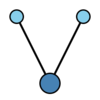
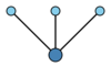
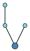
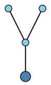
The rooted trees with at most four nodes are displayed in the table below.
| $t_1$ |
$t_2=[t_1]$ |
$ t_{3} = [t_{1},t_{1}]$ |
$t_4 = [t_2]$
|
 |
 |
 |

|
| $t_5 =[t_1,t_1,t_1]$ |
$t_6=[t_2,t_1]$ |
$ t_{7} = [t_{3}]$ |
$ t_{8} = [t_4]$
|
 |
 |
 |

|
Using this bracket notation for rooted trees, one can recursively define elementary differentials, as follows. Let
$$
F ( \emptyset ) ( y ( x ) ) = y ( x ) , \quad F ( \bullet ) ( y ( x ) ) = f ( y ( x ) ) ,
$$
and, for $ t = [ t _ {1} \dots t _ {m} ] $
with $ \rho ( t _ {i} ) \geq 1 $
for $ i = 1 \dots m $,
$$
F ( t ) ( y ( x ) ) =
$$
$$
=
f ^ {( m ) } ( y ( x ) ) ( F ( t _ {1} ) ( y ( x ) ) \dots F ( t _ {m} ) ( y ( x ) ) ) ,
$$
where $ f ^ {( m ) } ( y ( x ) ) $,
the $ m $
th derivative of $ f $
with respect to $ y $,
is a multi-linear mapping.
Since $ y ( x ) $
satisfies $ y ^ \prime ( x ) = f ( y ( x ) ) $,
it is not hard to show that
$$
y ^ {( i ) } ( x ) = \sum _ {t \in T _ {i} } \alpha ( t ) F ( t ) ( y ( x ) ) ,
$$
where $ y ^ {( i ) } ( x ) $
is the $ i $
th derivative of $ y $
with respect to $ x $,
$ T _ {i} = \{ {t \in T } : {\rho ( t ) = i } \} $,
and $ \alpha ( t ) $
is the number of distinct ways of labeling the nodes of $ t $
with the integers $ \{ 1 \dots \rho ( t ) \} $
such that the labels increase as you follow any path from the root to a leaf of $ t $.
Consequently, one can write the Taylor series for $ y ( x ) $
as a Butcher series:
\begin{equation}
\label{eq:1}
y ( x + h ) = \sum _ {i = 0 } ^ \infty y ^ {( i ) } ( x ) {
\frac{h ^ {i} }{i! }
} =
\end{equation}
$$
=
\sum _ {t \in T } \alpha ( t ) F ( t ) ( y ( x ) ) {
\frac{h ^ {\rho ( t ) } }{\rho ( t ) ! }
} .
$$
The importance of Butcher series stems from their use to derive and to analyze numerical methods for differential equations. For example, consider the $ s $-
stage Runge–Kutta formula (cf. Runge–Kutta method)
\begin{equation}\label{eq:2}
y _ {n + 1 } = y _ {n} + h \sum _ {i = 1 } ^ { s } b _ {i} k _ {i} ,
\end{equation}
$$
k _ {i} = f \left ( y _ {n} + h \sum _ {j = 1 } ^ { s } a _ {ij } k _ {j} \right ) ,
$$
for the ordinary differential equation $ y ^ \prime ( x ) = f ( y ( x ) ) $.
Let $ b = ( b _ {1} \dots b _ {s} ) ^ {T} \in \mathbf R ^ {s} $
be the vector of weights and $ A = [ a _ {ij } ] \in \mathbf R ^ {s \times s } $
the coefficient matrix for (a2). Then it can be shown that $ y _ {n + 1 } $
can be written as the Butcher series
\begin{equation}\label{eq:3}
y _ {n + 1 } = \sum _ {t \in T } \alpha ( t ) \psi ( t ) F ( t ) ( y _ {n} ) {
\frac{h ^ {\rho ( t ) } }{\rho ( t ) ! }
} ,
\end{equation}
where the coefficients $ \psi(t) \in \mathbf R $,
defined below, depend only on the rooted tree $t$
and the coefficients of the formula \eqref{eq:2}.
To define $ \psi ( t ) $,
first let
$$
\phi ( \emptyset ) = ( 1 \dots 1 ) ^ {T} \in \mathbf R ^ {s} ,
$$
$$
\phi ( \bullet ) = A \phi ( \emptyset ) ,
$$
and then, for $ t = [ t _ {1} \dots t _ {m} ] $
with $ \rho ( t _ {i} ) \geq 1 $
for $ i = 1 \dots m $,
define $ \phi ( t ) $
recursively by
$$
\phi ( t ) = \rho ( t ) A ( \phi ( t _ {1} ) \dots \phi ( t _ {m} ) ) ,
$$
where the product of $ \phi $'s in the bracket is taken component-wise. Then
$$
\psi ( \emptyset ) = 1,
$$
$$
\psi ( \bullet ) = \sum _ {i = 1 } ^ { s } b _ {i} ,
$$
and, for $ t = [ t _ {1} \dots t _ {m} ] $
with $ \rho ( t _ {i} ) \geq 1 $
for $ i = 1 \dots m $,
$$
\psi ( t ) = \rho ( t ) b ^ {T} ( \phi ( t _ {1} ) \dots \phi ( t _ {m} ) ) ,
$$
where, again, the product of $ \phi $'s in the bracket is taken componentwise.
Assuming that $ y ( x ) = y _ {n} $
and that $ \psi ( t ) = 1 $
for all trees $ t $
of order $ \leq p $,
it follows immediately from \eqref{eq:1} and \eqref{eq:3} that
$$
y _ {n + 1 } = y ( x + h ) + {\mathcal O} ( h ^ {p + 1 } ) .
$$
The order of \eqref{eq:2} is the largest such $p$.
Algebraic aspects
The Butcher series form a group, as they can be composed. This group is sometimes considered from the viewpoint of its Hopf algebra of functions.
The modern understanding of this notion uses the notion of pre-Lie algebras, for the following reasons:
- The Lie algebra of analytic vector fields on the affine space $\RR^d$ comes by anti-symmetrization from the pre-Lie product given by the usual torsion-free and flat connection.
- The free pre-Lie algebra on one generator can be described as the vector space spanned by rooted trees, under some kind of grafting.
Then, by the universal property of free pre-Lie algebras, the choice of any analytic vector field defines uniquely a morphism of pre-Lie algebras, which gives the "elementary differentials" associating a vector field to each rooted tree.
References
| [a1] | J.C. Butcher, "The numerical analysis of ordinary differential equations" , Wiley (1987) Zbl 0616.65072 |
| [a2] | E. Hairer, S.P. Nørsett, G. Wanner, "Solving ordinary differential equations I: nonstiff problems" , Springer (1987) Zbl 0638.65058 |


